Tag: base

Multipath and Antenna Selection

1. Introduction

Multipath is an important local error source in Global Navigation Satellite System (GNSS) measurements. It occurs when signals reach an antenna through both a direct path and one or more reflected or diffracted paths. Unlike many satellite orbit, satellite clock and atmospheric errors—which may be partly mitigated through differencing, estimation or correction models—multipath is strongly dependent on the antenna’s immediate surroundings and can differ substantially between installations.

Antenna design and installation are the first lines of defence. Antenna gain patterns and polarisation characteristics can attenuate some reflected signals before they enter the receiver. Receiver tracking and estimation algorithms can provide additional mitigation, but neither antenna design nor receiver processing can guarantee the removal of all multipath.

The appropriate antenna therefore depends on the application, required accuracy, signal bands, operating environment, installation constraints and calibration requirements. These factors are particularly important for RTK, surveying, geodetic monitoring and precision timing.

2. What is multipath?

Multipath occurs when a receiver processes a GNSS signal that contains the direct line-of-sight component together with delayed copies reflected from surfaces such as buildings, the ground, water, vehicles, solar panels or parts of the platform carrying the antenna. The additional path length introduces a delay; the reflected component also has a relative phase and amplitude that depend on the geometry and reflecting surface.

The receiver processes the composite signal. The reflected component can distort code-tracking correlation functions and perturb carrier-phase tracking, producing measurement errors. The magnitude and time variation of those errors depend on the signal waveform, excess path delay, relative amplitude and phase, antenna response, receiver bandwidth and tracking-loop or correlator design.

2.1 Effects on code and carrier-phase measurements

Code pseudorange: Multipath can shift the estimated code-tracking point. Errors range from small values to metres or more in adverse conditions; no single range is a universal upper bound for all signals, geometries and receiver designs.
Carrier phase: Multipath perturbs the measured carrier phase and can produce errors at the millimetre-to-centimetre scale in many precision applications. For a simplified single-reflection model, the phase error is commonly described as having a theoretical maximum of approximately one quarter of a carrier wavelength. This is about 4.8 cm at GPS L1 and 6.1 cm at GPS L2 when expressed as range-equivalent phase error. Real behaviour depends on the reflected signal and tracking conditions.

The following table gives qualitative guidance, not guaranteed performance limits.

Measurement or signal	General behaviour	Important qualification
Code on GPS L1 C/A	Can be strongly affected by multipath; errors may range from small values to metres in difficult environments.	Actual error depends on excess delay, reflection strength, waveform and receiver correlator.
Code on wider-band signals such as GPS L5 and Galileo E5	Generally offers better intrinsic code-multipath performance for comparable conditions.	Performance is signal- and receiver-dependent; wider bandwidth does not eliminate multipath.
Carrier phase	Often supports very precise measurements, but multipath can still cause millimetre-to-centimetre errors and affect ambiguity resolution.	The quarter-wavelength figure is a simplified theoretical bound, not a guaranteed bound on the final position solution.

GPS L5 has a chipping rate of 10.23 Mchip/s, corresponding to a chip duration of approximately 97.8 ns and a propagation distance of about 29.3 m per chip. Galileo E5 uses wideband AltBOC(15,10) modulation. These signal properties support sharper correlation features and generally improve code-multipath resistance, particularly for short-delay reflections. The receiver’s actual tracking architecture remains important.

2.2 Factors that influence multipath severity

Reflector geometry and excess path delay: Nearby surfaces can create short-delay reflections that are difficult to distinguish from the direct signal. Longer-delay reflections may be easier for some specialised receiver algorithms to identify, but this is not guaranteed.
Satellite elevation and azimuth: Low-elevation signals often encounter more local obstructions and reflecting surfaces, although multipath can affect satellites at higher elevations too. Elevation masking can reduce some errors but also reduces satellite availability and may worsen geometry.
Signal waveform and receiver tracking: Signal bandwidth, modulation, correlator spacing, tracking-loop design and multipath-mitigation algorithms all influence the resulting measurement error.
Reflection properties and polarisation: GNSS satellite signals are transmitted with right-hand circular polarisation (RHCP). A simple specular reflection can reverse circular-polarisation sense, but real surfaces and geometries may produce mixed polarisation. Antenna discrimination between RHCP and LHCP can help reject some reflected energy, but the benefit depends on angle, frequency and antenna design.
Platform and installation: Roofs, vehicle bodies, masts, radomes, cables and nearby equipment can alter the antenna pattern or create additional reflections. The installation can therefore behave differently from the antenna measured in isolation.

3. Direct and reflected signal paths

Figure 1. The antenna receives the direct signal together with delayed reflected components. Their amplitudes, delays, phases and polarisation states depend on the reflecting surfaces and geometry.

4. How antenna design can reduce multipath

An antenna does not normally identify a reflection by its delay. Instead, its spatial response and polarisation characteristics can attenuate some signals according to their arrival direction and polarisation. Receiver processing may then provide further mitigation.

Gain pattern and low-elevation response: Antennas designed for surveying often control gain near and below the horizon to reduce sensitivity to some ground and nearby-structure reflections. The trade-off is reduced reception of low-elevation satellites. The actual elevation-dependent gain pattern should be examined rather than inferred from the antenna category.
Polarisation purity and axial ratio: Good RHCP performance and appropriate RHCP-to-LHCP discrimination can reduce the impact of some reflections. Axial ratio describes how closely the polarisation approximates circular polarisation; it is not, by itself, a complete measure of multipath rejection. Performance varies with frequency, azimuth and elevation.
Ground plane: A suitable conductive ground plane can modify the radiation pattern and reduce reception from below, depending on its dimensions, geometry and mounting. Its edges can also cause diffraction, so the result is design-dependent.
Choke rings: Concentric conductive grooves around a geodetic antenna element are designed to suppress surface currents and reduce low-elevation and ground-reflected signals. Choke-ring antennas are widely used at high-precision reference stations because of their stable, well-characterised behaviour and strong multipath mitigation. They are larger, heavier and generally more expensive than compact antennas; they are not automatically optimal for every installation.
Phase-centre behaviour: The antenna’s effective phase centre varies with signal direction and frequency. Phase-centre offset (PCO) is the mean offset from the antenna reference point; phase-centre variation (PCV) describes changes around that model. For high-precision work, use suitable calibration data and apply the correct antenna model consistently. Calibration corrects antenna phase-centre behaviour; it does not remove arbitrary site multipath.
Controlled-reception-pattern antenna (CRPA): A multi-element array can adapt its reception pattern to suppress signals arriving from selected directions. CRPAs are primarily used for interference and jamming mitigation. They may affect multipath in some circumstances, but they should not be treated as a general substitute for multipath-resistant antenna design and good siting.

Antenna calibration performed in a chamber characterises the antenna under controlled conditions. Nearby structures and the installed mounting configuration can still change the effective pattern and create site-specific multipath. For demanding applications, the complete antenna, mount, radome and installation should be considered.

5. Antenna types: practical comparison

Antenna type	Typical strengths	Typical applications and caveats
Compact patch (passive or active)	Small, low-cost and easy to integrate; performance varies widely by design and ground plane.	Consumer devices, asset tracking and embedded products. Do not assume precision multipath performance from size or band count alone.
Multi-band patch or helical	Can support multiple constellations and bands in a compact package; performance depends strongly on design and installation.	Drones, vehicles, robotics and compact precision systems. Verify phase-centre and low-elevation performance if accuracy demands it.
Survey/precision antenna with ground plane	Designed for more controlled gain and phase-centre behaviour than many compact antennas.	RTK rovers, machine control and surveying. Check calibration, mounting requirements and performance in the intended environment.
Choke-ring geodetic antenna	Strong multipath mitigation and well-established use in high-precision reference installations.	CORS and geodetic monitoring. Larger, heavier and more costly; select a calibrated model appropriate to the signals tracked.
Timing antenna	May be optimised for stable reception, suitable gain and fixed-site operation.	Timing receivers and synchronisation installations. Timing performance also depends on receiver design, sky visibility, antenna delay stability and installation.
CRPA / adaptive antenna array	Can form spatial nulls towards selected interference sources.	Jamming and interference resilience. More complex and not primarily a general-purpose multipath solution.

These categories are only a first screening tool. Compare measured gain patterns, polarisation performance, calibration data, supported frequencies, environmental ratings and test results for the specific antenna model.

6. Selection and installation

6.1 What to check in the datasheet

Frequency and constellation coverage: Confirm support for every signal the receiver is intended to use, including the required L-band signals and any relevant E6 or BeiDou B3 signals. Check the exact frequency bands and polarisation requirements, not just a generic ‘multi-GNSS’ label.
Radiation pattern: Review gain versus elevation and, where available, azimuth-dependent plots. Check low-elevation behaviour and performance below the horizon where relevant.
Polarisation: Review axial-ratio and polarisation-discrimination data across the required bands and angular range. A single zenith value is not enough to characterise performance.
Calibration: For centimetre-level or geodetic work, confirm that suitable absolute antenna calibration data are available in the format and convention required by the processing workflow. Ensure the antenna model and processing corrections are consistent.
Reference point: Understand how the manufacturer defines the antenna reference point and phase-centre offsets. Apply the correct offsets and variations in the receiver or post-processing software.
LNA, noise figure and filtering: For active antennas, confirm that gain is appropriate for cable loss and receiver input requirements. Consider noise figure, current consumption, out-of-band filtering and susceptibility to nearby interference. Excessive gain can overload a receiver front end.
Mechanical and environmental suitability: Check mounting, connector type, cable routing, weatherproofing, vibration, temperature range and radome requirements. Confirm whether the published performance assumes a specific ground plane or mounting arrangement.

6.2 Installation practice

Sky visibility: Choose a location with a clear sky view and minimal obstructions. Avoid nearby walls, parapets, metal roof edges, fences, solar panels and other reflective surfaces where practical.
Reflector clearance: Keep the antenna away from large reflective surfaces and platform edges where the application permits. There is no universal minimum separation distance: the impact depends on reflector geometry, antenna pattern and required performance.
Mounting stability: Use a rigid, stable mount. For reference stations, account for monument stability, thermal expansion, wind loading and long-term movement.
Ground plane and mounting surface: Follow the antenna manufacturer’s specified mounting configuration. A ground plane can improve performance for some antennas, but adding one arbitrarily may alter the pattern and calibration.
Orientation and reference point: Follow manufacturer and processing requirements for antenna orientation. For high-precision geodetic stations, document the antenna reference point, monument eccentricities, antenna model, radome and orientation consistently in station metadata and observation files.
Cable, connectors and protection: Use cable with suitable loss at the operating frequencies, weatherproof connectors and appropriate grounding, surge and lightning protection. Keep cable routing and nearby electronics from introducing interference.
Verification after installation: Inspect satellite C/N0 by elevation and azimuth, tracking continuity, code-minus-carrier or other receiver multipath indicators, measurement residuals and position repeatability. Compare results across time and satellite geometry. No single diagnostic metric proves that multipath is absent.

7. A practical selection workflow

A defensible antenna choice follows the application rather than a generic ranking of antenna types:

Define the required position or timing performance and the operating environment.
List the GNSS constellations, frequencies and signals the receiver will use.
Assess nearby reflectors, sky visibility, platform effects, cable loss and interference risks.
Shortlist antennas with appropriate radiation patterns, polarisation performance and environmental ratings.
For precision applications, verify calibration availability and compatibility with the intended processing chain.
Test the antenna in the actual mounting configuration and assess measurement quality and repeatability.

8. Conclusion

Reliable GNSS performance depends on the receiver, antenna and installation working together. Wider-band signals can improve intrinsic code-multipath resistance, while antenna patterns and polarisation characteristics can reduce some reflected energy. Precision antennas and suitable calibration are particularly important for RTK, surveying and geodetic applications, but calibration does not eliminate site-specific multipath.

The strongest engineering approach is to select an antenna for the actual signals and environment, install it with a clear sky view and stable mounting, apply the correct calibration model, and verify performance using receiver diagnostics and repeatable measurements. Choke-ring antennas are a strong option for many geodetic reference stations, whereas compact patches or other antennas may be more appropriate for size-, weight- or cost-constrained products.

Technical references and further reading

International GNSS Service (IGS), Antenna Committee and antenna calibration resources. https://www.igs.org/wg/antenna/
IGS CORS Guidelines, GNSS antenna. https://igs.git-pages.gfz-potsdam.de/igs-cors-guidelines/en/equipment/antenna/
IGS CORS Guidelines, signal quality and multipath. https://igs.git-pages.gfz-potsdam.de/igs-cors-guidelines/en/establishment/signals/
NOAA National Geodetic Survey, GNSS antenna calibration. https://nweb.ngs.noaa.gov/research/gnss-satellite/gnss-antenna-calibration.shtml

Lau and Cross (2007), Development and testing of a new ray-tracing approach to GNSS carrier-phase multipath modelling, Journal of Geodesy.

https://doi.org/10.1007/s00190-007-0139-z

For more support contact us at: info@linfinitygnss.com

1. Introduction Multipath is an important local error source in Global Navigation Satellite System (GNSS) measurements. It occurs when signals reach an antenna through both a direct path and one or more reflected or diffracted paths. Unlike many satellite orbit, satellite clock and atmospheric errors—which may be partly mitigated through differencing, estimation or correction models—multipath…

October 10, 2026

Satellite Orbits and GNSS Constellations

A technical guide to where navigation satellites fly, why, and how augmentation systems sharpen the result.

1. Introduction

Every position fix a GNSS receiver produces relies on signals from satellites more than 20,000 km away, each travelling at close to 4 km/s. The receiver can only turn those signals into an accurate position fix if it knows exactly where each satellite was when it transmitted. The design of GNSS orbits, and how precisely they are known, therefore has a direct effect on the accuracy, availability and integrity that users see on the ground.

2. What is a GNSS orbit?

A GNSS orbit is the specific path that a Global Navigation Satellite System (GNSS) satellite follows as it travels around the Earth while broadcasting precise positioning and timing signals.

GNSS satellites provide the reference position and time needed for positioning measurements. A receiver estimates its position by measuring the propagation time of signals from multiple satellites whose positions are known or precisely modelled. Errors in the estimated satellite positions therefore contribute directly to the user’s positioning error. For this reason, GNSS satellite orbits are designed to be stable and predictable, and they are continuously monitored and determined by ground control networks.

Most GNSS satellites operate in medium Earth orbit (MEO), at altitudes of approximately 19,000-23,500 km. Examples include GPS at around 20,200 km, GLONASS at around 19,100 km, Galileo at approximately 23,222 km, and BeiDou’s MEO satellites at approximately 21,528 km. At these altitudes, a satellite completes one revolution in roughly 11-14 hours.

At MEO altitudes, each satellite can be visible over a large portion of the Earth’s surface. By deploying multiple satellites in carefully designed orbital planes, GNSS constellations provide continuous or near-continuous satellite visibility over most of the globe, with sufficient satellite geometry to support positioning. In open-sky conditions, users can typically observe several satellites simultaneously.

Some systems also use geostationary (GEO) or inclined geosynchronous (IGSO) orbits to enhance regional coverage. BeiDou uses GEO, IGSO and MEO satellites, while QZSS and NavIC use combinations of MEO and geosynchronous orbits, including IGSO, to improve coverage over their target regions.

2.1 Describing a GNSS orbit

Six parameters, known as the Keplerian elements, fully define a GNSS orbit:

Semi-major axis – sets the orbit’s size and therefore its period. For GPS, this gives a period of half a sidereal day (about 11 h 58 min), so the same satellite geometry repeats over a given location every day, roughly four minutes earlier each time.
Eccentricity – GNSS orbits are designed to be near-circular (e < 0.02), keeping altitude, signal power and Doppler behaviour predictable.
Inclination – around 55-56° for GPS, Galileo and BeiDou MEO, and 64.8° for GLONASS, which improves visibility at high latitudes.
RAAN (right ascension of the ascending node) – orients each orbital plane in space. Spreading satellites across several planes (six for GPS, three for GLONASS, Galileo and BeiDou MEO) is what gives global coverage.
Argument of perigee and mean anomaly – fix the satellite’s position within its plane at a reference time.

These elements, plus perturbation corrections, are broadcast in the navigation message as the ephemeris. From them, a receiver computes each satellite’s position to about 1 m, and that accuracy feeds directly into every range measurement.

3. The main orbit families

The orbit chosen for a satellite depends on its mission: the required coverage, visibility, revisit time, orbital period, and distance from Earth.

Figure 1 – the main orbit families: LEO, MEO, GEO/IGSO, the polar/Sun-synchronous orbit shown edge-on, and the GTO transfer ellipse between LEO and GEO.

Figure 2 — Representative altitudes on a logarithmic scale. GNSS constellations cluster in MEO between about 19,000 and 23,500 km.

GNSS constellations cluster in MEO, between about 19,000 and 23,500 km, well above LEO and well below the geostationary belt at 35,786 km.

3.1 Low Earth orbit (LEO)

LEO covers altitudes from roughly 160 km up to about 2,000 km, although most LEO missions operate below 1,000 km. Satellites in LEO travel at around 7.8 km/s and typically complete an orbit in about 90 minutes. The International Space Station, at an altitude of roughly 420 km, orbits Earth about 16 times per day. For comparison, commercial airliners typically cruise at around 11-12 km, so even the lowest operational orbits are more than ten times higher.

The proximity to Earth makes LEO particularly attractive for high-resolution Earth observation and crewed missions. LEO satellites can operate at a wide range of orbital inclinations, depending on the mission requirements. The trade-off is a relatively small coverage area and short visibility periods: a single LEO satellite passes across the sky in minutes, so continuous or near-continuous services generally require large constellations.

LEO is also attracting growing interest for positioning, navigation and timing (PNT), both through dedicated augmentation signals and as a complementary layer to traditional MEO GNSS. The lower altitude can provide stronger received signals and faster-changing geometry, potentially offering benefits for positioning performance and resilience.

3.2 Medium Earth orbit (MEO)

MEO occupies the region between LEO and geostationary orbit, generally from about 2,000 km to 35,786 km above Earth’s surface. It is the primary orbital regime used by the global navigation constellations – GPS, Galileo, GLONASS and the MEO component of BeiDou – because it offers a good balance between coverage, signal strength and constellation size.

MEO satellites typically have orbital periods of roughly 11 to 14 hours, depending on their altitude. Their movement across the sky provides continuously changing satellite geometry, which is important for accurate positioning. Because each satellite covers a relatively large area of Earth, global or near-global coverage can be achieved with constellations of roughly 24 or more satellites when they are distributed across suitable orbital planes. The exact number and orbital geometry depend on the design of each GNSS constellation.

BeiDou is somewhat different from the other global GNSS because, in addition to its MEO satellites, it also uses satellites in geostationary (GEO) and inclined geosynchronous (IGSO) orbits to provide additional regional coverage and system capabilities.

3.3 Geostationary orbit (GEO)

A geostationary satellite orbits at an altitude of approximately 35,786 km above the equator and travels eastward at about 3.07 km/s. It completes one orbit in one sidereal day (23 h 56 min 4 s), matching the rotation period of Earth relative to the stars. As a result, it remains above approximately the same point on the equator and appears fixed in the sky to an observer on the ground. Ground antennas can therefore be pointed at a fixed position without needing to track the satellite.

This makes GEO particularly valuable for broadcasting, telecommunications, continuous weather monitoring and certain satellite-based augmentation system (SBAS) services. Because of its great altitude, a single GEO satellite can see roughly one-third of Earth’s surface, although the exact coverage depends on the satellite’s field of view and the minimum elevation angle required by the service. A small number of suitably positioned GEO satellites can therefore provide coverage over most of the populated regions of the world, but coverage becomes increasingly limited at high latitudes and near the poles.

The main disadvantages of GEO are the long signal propagation delay, low elevation angles at high latitudes, and the limited number of usable orbital positions along the equatorial geostationary belt. The large distance also results in higher free-space path loss and weaker received signals compared with satellites in lower orbits.

3.4 Inclined geosynchronous orbit (IGSO)

An IGSO is a geosynchronous orbit whose orbital plane is inclined relative to the equator. For a circular IGSO, the satellite’s ground track forms a characteristic north-south figure-of-eight pattern as seen from Earth. The inclination determines the north-south extent of the ground track, while orbital eccentricity can further modify its shape and the amount of time the satellite spends over particular regions.

IGSO satellites are used by navigation systems such as BeiDou and NavIC, while Japan’s QZSS uses geosynchronous and other specially designed orbits to maintain high-elevation coverage over Japan and the Asia-Pacific region. These orbits can provide satellites that remain visible at relatively high elevation angles for extended periods, which is particularly valuable in environments where surrounding buildings or terrain obstruct lower-elevation signals, such as urban canyons and mountainous areas.

3.5 Polar and Sun-synchronous orbits (SSO)

Polar orbits are highly inclined orbits that pass over or near the polar regions, with an inclination close to 90°. They can operate at a wide range of altitudes, although many Earth-observation satellites operate in LEO, typically at altitudes of around 500-800 km. As the satellite orbits Earth while the Earth rotates beneath it, successive passes follow different ground tracks, allowing the satellite to build up coverage of much of the planet.

A Sun-synchronous orbit (SSO) is a special type of near-polar orbit, typically used at altitudes of several hundred kilometres, whose orbital plane slowly precesses at approximately the same rate as the Sun’s apparent annual motion. This means that the satellite crosses a given latitude at approximately the same local solar time on successive passes. The resulting consistency in solar illumination makes images acquired on different days, seasons and years more directly comparable. SSOs are therefore widely used for Earth observation, including applications such as crop monitoring, land-use mapping and flood assessment.

Dawn-dusk Sun-synchronous orbits are designed so that the satellite remains close to the day-night terminator. This can keep the spacecraft in sunlight for most or all its orbit, providing favourable conditions for solar-power generation and reducing the time spent in Earth’s shadow.

3.6 Orbit comparison at a glance

Orbit	Typical altitude	Period	Typical uses
LEO	160-2,000 km	~90-120 min	Imaging, crewed stations, broadband constellations, LEO-PNT
SSO (LEO subset)	600-800 km	~100 min	Earth observation with constant lighting
MEO	2,000-35,786 km	~2-24 h	GNSS (GPS, Galileo, GLONASS, BeiDou)
GEO	35,786 km (equatorial)	23 h 56 min	Communications, weather, SBAS, BeiDou GEO
IGSO	35,786 km (inclined)	23 h 56 min	Regional navigation (BeiDou, QZSS, NavIC)
GTO	~200 x 35,786 km	~10.5 h	Transfer to GEO
L1 / L2	~1.5 million km	Halo orbit	Solar and deep-space observatories

4. GNSS constellations

A receiver needs signals from at least four satellites to solve for its three-dimensional position and its receiver clock offset. Constellation designers therefore distribute satellites across multiple orbital planes and carefully chosen orbital positions so that, from almost anywhere on Earth, sufficient satellites are visible above the receiver’s elevation mask with good geometric distribution across the sky.

Using multiple GNSS constellations together increases the number and diversity of visible satellites. This can improve satellite geometry and positioning robustness, accelerate convergence for high-precision techniques such as RTK and PPP, and maintain service availability when buildings, terrain or other obstructions block part of the sky.

4.1 GPS (United States)

GPS satellites operate in MEO at an altitude of approximately 20,200 km. Each satellite completes an orbit in about 11 hours 58 minutes, or roughly two orbits per sidereal day. The GPS baseline constellation consists of 24 slots arranged in six equally spaced orbital planes, with four slots in each plane and an inclination of 55°. This geometry is designed to provide at least four satellites in view from virtually any point on Earth.

In practice, the U.S. Space Force operates more than the 24-satellite baseline. These additional satellites provide redundancy, helping maintain coverage when satellites are unavailable for maintenance or are retired, and can also improve constellation geometry and positioning performance. They are generally referred to as auxiliary or additional satellites rather than part of the baseline 24-slot constellation.

4.2 Galileo (European Union)

Galileo satellites operate in MEO at an altitude of approximately 23,222 km, in three orbital planes inclined at 56° to the equator. Each satellite takes about 14 hours to complete an orbit. The nominal constellation is a 24/3/1 Walker configuration, with 24 nominal satellites distributed across the three planes; additional satellites can serve as in-orbit spares and be repositioned to replace satellites that are unavailable.

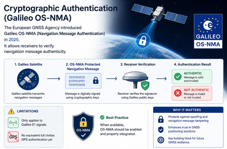
Galileo provides the Open Service (OS) for free positioning and timing, the High Accuracy Service (HAS), which is freely available and provides PPP corrections for improved real-time positioning, and Open Service Navigation Message Authentication (OSNMA), which allows receivers to authenticate Galileo navigation data and helps protect against spoofing. OSNMA was declared operational on 24 July 2025.

4.3 GLONASS (Russia)

GLONASS satellites operate in MEO at an altitude of approximately 19,100 km, in three orbital planes inclined at 64.8° to the equator. Each satellite completes an orbit in roughly 11 hours 15 minutes. The relatively high orbital inclination gives GLONASS good satellite visibility at high northern and southern latitudes, making it particularly well suited to users in regions where lower-inclination constellations provide less favourable satellite geometry.

The GLONASS constellation is designed around 24 operational satellite slots, with eight satellites nominally distributed in each of the three orbital planes.

4.4 BeiDou (China)

BeiDou-3 uses a hybrid constellation of three orbit types: 24 MEO satellites at approximately 21,528 km, inclined at 55°; 3 IGSO satellites at 35,786 km, also inclined at 55°; and 3 GEO satellites at 35,786 km, positioned at 80°E, 110.5°E and 140°E. Spare satellites can also be deployed in orbit as required.

The MEO satellites provide the global backbone of the constellation, while the GEO and IGSO satellites provide additional high-elevation visibility and service capability over the Asia-Pacific region. This hybrid architecture is one of the defining characteristics of BeiDou and allows it to combine global MEO coverage with enhanced regional coverage and services.

4.5 Regional systems

Two regional systems complement the global constellations. Japan’s QZSS uses quasi-zenith and geostationary orbits to keep at least one satellite close to overhead in Japan, improving availability in dense cities and supporting augmentation services. India’s NavIC uses GEO and IGSO satellites to provide positioning over India and the surrounding region; the nominal constellation design and current operational satellite status can differ.

4.6 Constellation comparison

System	Orbit(s)	Altitude	Inclination	Planes / slots	Period (MEO)
GPS	MEO	20,200 km	55°	6 planes, 24 baseline slots	11 h 58 min
Galileo	MEO	23,222 km	56°	3 planes, 24 operational + 3 spares	14 h 05 min
GLONASS	MEO	19,100 km	64.8°	3 planes, 24 satellites	11 h 15 min
BeiDou-3	MEO + IGSO + GEO	21,528 km (MEO); 35,786 km (IGSO/GEO)	55° (MEO/IGSO), 0° (GEO)	24 MEO + 3 IGSO + 3 GEO	~12 h 53 min
QZSS	IGSO + GEO	~35,786 km*	~40° (IGSO), 0° (GEO)	Regional	–
NavIC	GEO + IGSO	~35,786 km	29° (IGSO), 0° (GEO)	Regional	–

*QZSS note: the inclined QZSS satellites are in elliptical geosynchronous orbits, so their altitude varies during each orbit. ~35,786 km is the reference altitude of a circular geostationary orbit, not the constant altitude of the inclined QZSS satellites.

Values are nominal constellation/design parameters; the number and operational status of satellites can change over time.

5. Satellite-based augmentation systems (SBAS)

GNSS augmentation improves the performance of standalone GNSS by providing additional information that allows the receiver to correct or bound errors in the positioning solution. This information can include estimates of satellite clock and orbit (ephemeris) errors, ionospheric delays, and integrity information indicating how large the remaining errors could be. Augmentation can also take the form of local corrections or external aiding, depending on the system. Augmentation systems are commonly classified according to how the additional information is delivered to the user.

SBAS provides wide-area corrections and integrity information, typically broadcast through geostationary satellites. A network of precisely surveyed reference stations continuously monitors the GNSS signals across a region. The measurements are sent to central processing facilities, which estimate satellite and atmospheric errors, generate corrections and integrity information, and send the resulting messages to uplink stations. These stations transmit the messages to geostationary satellites, which broadcast them over the service area on standardised GNSS-compatible signals. An SBAS-capable receiver within the coverage area can use the augmentation data without a separate subscription.

Beyond accuracy, SBAS supplies integrity: timely warnings when a satellite or correction should not be trusted, together with protection levels that bound the position error. This is why SBAS is certified for aircraft approach guidance and is widely used in agriculture, maritime, surveying and road applications.

Operational and developing SBAS include:

WAAS – United States
EGNOS – Europe
MSAS – Japan
GAGAN – India
SDCM – Russia
BDSBAS – China
KASS – South Korea
SouthPAN – Australia and New Zealand

6. Why this matters for GNSS users

For anyone designing or deploying a positioning solution, the space segment has direct, practical consequences:

More constellations, more satellites. Tracking GPS, Galileo, GLONASS and BeiDou together typically puts several dozen satellites in view, improving geometry, availability and redundancy, and increasing resilience in obstructed environments.
Orbit design drives local performance. High-inclination GLONASS helps at northern latitudes; IGSO satellites from BeiDou and QZSS add high-elevation signals in the Asia-Pacific region.
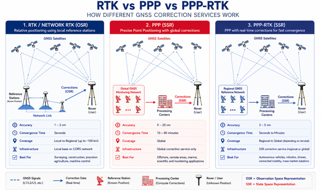
Augmentation closes the gap. SBAS can improve accuracy and provide integrity information, while PPP and RTK services can deliver sub-metre to centimetre-level positioning depending on the service, receiver and operating conditions.
New layers are coming. LEO-based positioning and correction services promise faster convergence and additional robustness alongside traditional MEO GNSS.

Linfinity GNSS works with customers to match receivers, antennas and correction services to the constellations and orbits that best serve their application. For further information, contact admin@linfinitygnss.com.

A technical guide to where navigation satellites fly, why, and how augmentation systems sharpen the result. 1. Introduction Every position fix a GNSS receiver produces relies on signals from satellites more than 20,000 km away, each travelling at close to 4 km/s. The receiver can only turn those signals into an accurate position fix if…

October 7, 2026

The cost of GNSS Reacquisition
The Hidden Power Cost of GNSS Reacquisition

infinitygnss.com

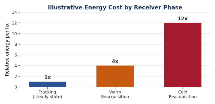
Most GNSS power budgets are built around the receiver’s steady-state tracking current — the datasheet number for “continuous tracking mode.” In the field, that number tells only part of the story. Every time a receiver loses lock and has to find its way back to a fix, it burns far more energy than it does while quietly tracking satellites it already knows about. For battery-powered trackers, wearables, and IoT nodes, this reacquisition penalty is often the single biggest, most overlooked drain on system lifetime.

Acquisition, Tracking, and Reacquisition
- Acquisition — the initial search phase. The receiver sweeps a two-dimensional space of frequency (Doppler) bins against code-phase bins for every satellite in view. Computationally heavy: many correlators, or many sequential search bins.
- Tracking — the steady state. A narrow loop follows small changes in Doppler and code phase, using a fraction of the correlator resources and power that acquisition needs.
- Reacquisition — acquisition’s less forgiving cousin, triggered mid-mission by a signal outage. It’s the phase that quietly dominates power budgets in real deployments.
I

Why Reacquisition Happens So Often
- Urban canyons and foliage repeatedly block and unblock line of sight as a device moves.
- Tunnels and building interiors cause complete signal loss for seconds to hours.
- Multipath / interference can drop carrier-to-noise ratio below the tracking threshold even with a nominally visible satellite.
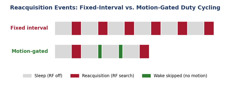
- Aggressive duty-cycling is itself a major cause: powering down the RF front end between fixes means every wake-up is, by definition, a reacquisition — not a continuation of tracking. This creates a direct tension: more aggressive duty-cycling means paying the larger reacquisition cost more often instead of the smaller tracking cost.
Where the Power Actually Goes
- Wider search space — no recent time/ephemeris estimate forces a full Doppler/code-phase sweep, orders of magnitude more correlator work than a warm reacquisition.
- Longer time-to-fix (TTFF) — more search bins and weaker signal both stretch active RF/baseband time, and therefore energy, per fix.
- Repeated partial searches — marginal conditions can cause several failed acquisition attempts before a stable fix, multiplying the energy cost.
- Ephemeris/almanac staleness — valid for ~2–4 hours; a longer sleep forces a full re-download (~18–30+ seconds) in a high-power state.
Duty-Cycling Smarter, Not Just Less

The tracking-vs-reacquisition trade-off is not a hard trade-off- it’s a design decision. A few techniques keep most of the standby savings while shrinking the reacquisition penalty per wake-up:
- Adaptive/variable intervals : shorten sleep when moving quickly (favouring cheap hot starts), lengthen it when stationary or predictable.
- Keeping time, not signal — a disciplined RTC/TCXO through sleep preserves time accuracy, narrowing the Doppler search on wake-up for very little standby current.
- Coarse signal-presence checks — a low-power pre-check before a full search avoids to do attempts when the antenna does not have a good sky view.
- Batching around known outages — scheduling wake-ups to avoid predictable blockage (a daily tunnel, an overnight indoor period).
- Hybrid tracking modes — an intermediate low-power lock state turns “reacquisition” into a cheap return to precision rather than a search from scratch.
Other Levers Worth Engineering For
- A-GNSS assistance data and extended/predicted ephemeris collapse the search space and avoid the re-download tax after long sleeps.
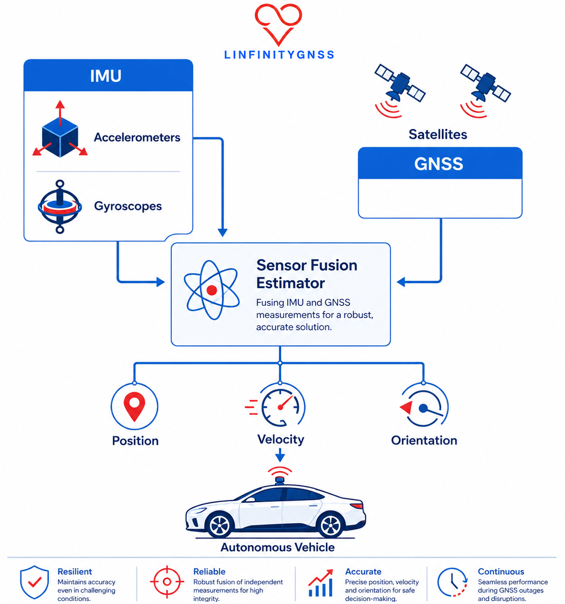
- Sensor fusion / dead reckoning bridges short outages and narrows the search space on wake-up.
- Multi-constellation, multi-frequency receivers and better antenna/RF quality reduce how often lock is lost in the first place — the cheapest fix of all.
The Takeaway

Datasheet tracking current says little about real-world battery life. Reacquisition frequency and cost are usually the real determinant. Power budgets for trackers, wearables, and IoT devices should be built around a realistic reacquisition rate for the target environment – and clever duty-cycling, assistance data, and sensor fusion should be treated as core power-management features, not optional ext
The Hidden Power Cost of GNSS Reacquisition infinitygnss.com Most GNSS power budgets are built around the receiver’s steady-state tracking current — the datasheet number for “continuous tracking mode.” In the field, that number tells only part of the story. Every time a receiver loses lock and has to find its way back to a fix,…

September 8, 2026

Anti-Jamming Antennas Explained:How CRPA, Receiver Mitigation and Monitoring Work Together

GNSS receivers are designed to recover extremely weak signals from satellites millions of kilometres away. That makes them inherently vulnerable to radio-frequency interference: a nearby interferer does not need to reproduce a GNSS signal to cause damage. It only needs to raise the interference environment at the receiver input enough to reduce tracking margin, desensitize the front end, or prevent acquisition and tracking altogether.

The engineering response is not simply to buy an “anti-jam antenna”. Resilient PNT is a system property. Antenna architecture, RF filtering, receiver dynamic range, interference detection, adaptive processing, firmware, installation, and—where required—independent sensors and holdover all contribute to the outcome.

This guide explains the differences between a conventional fixed-reception-pattern antenna (FRPA), pattern-shaped antennas, and controlled-reception-pattern antennas (CRPAs); explains why CRPA performance depends on the antenna electronics and receiver architecture; and provides a practical framework for selecting the appropriate level of protection.

1. Standard Antennas vs. Anti-Jamming Antennas: What Actually Changes?

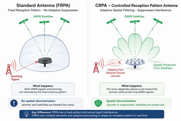
A conventional GNSS antenna has a fixed spatial reception pattern. It may be a simple patch, a more sophisticated precision antenna, or a multi-band design with filtering and a low-noise amplifier. Its pattern is determined by the antenna geometry, ground plane, radome, installation, and RF design. Once manufactured and installed, that pattern does not adapt in real time to the direction of an interferer.

That distinction matters because the antenna does not intrinsically know whether an RF signal is legitimate or hostile. A jammer arriving from an azimuth and elevation inside the antenna’s useful reception region is simply another RF input. If the interference is strong enough, the receiver may lose carrier tracking, suffer front-end compression or saturation, or experience a rise in the effective noise floor.

A CRPA takes a fundamentally different approach. Instead of relying on a single antenna element, it uses multiple spatially separated elements whose signals are processed coherently. The system can estimate the spatial characteristics of interference and apply complex weights to the element signals. The resulting array response can place deep spatial nulls toward one or more interferers while retaining useful sensitivity to GNSS signals.

The important point is that a CRPA does not simply ‘block the jammer’. It changes the spatial weighting of the received signals before the receiver processes them as GNSS measurements. The exact architecture varies between products: some systems emphasize null steering, some combine nulling and beamforming, and some integrate additional interference detection or filtering.

Figure 1 — Fixed reception versus adaptive spatial filtering. The CRPA concept is shown as an adaptive spatial response with a null directed toward the interferer.

One terminology point is worth making: an FRPA should not be described as having ‘equal gain in every direction’. Real GNSS antennas have elevation and azimuth-dependent gain, polarization characteristics, multipath sensitivity, and often deliberate pattern shaping. The defining property of an FRPA is that its spatial response is fixed—not that it is perfectly isotropic.

2. There Is a Middle Ground: Pattern-Shaped Antennas

Between a conventional antenna and a full CRPA there are antennas designed to reduce interference through a fixed spatial pattern. Choke rings, optimized ground planes, low-elevation suppression, and out-of-band filtering can all reduce the amount of unwanted energy reaching the receiver.

This works well when the interference geometry is predictable. For example, suppressing low-elevation signals can reduce the impact of a ground-based jammer while preserving most of the useful GNSS sky view.

But the pattern is fixed. If the jammer moves, the antenna cannot move the rejection zone with it. Pattern shaping reduces vulnerability by design; a CRPA adapts to the interference in real time.

Architecture	Spatial response	Interference discrimination	Typical complexity
FRPA	Fixed	None beyond the inherent antenna pattern	Low
Pattern-shaped antenna	Fixed, deliberately shaped	Limited and geometry-dependent	Low–moderate
CRPA	Adaptive	Dynamic nulling and/or beamforming	Moderate–high

3. Why the Antenna Is Only Part of the Anti-Jam System

The term anti-jam antenna can be misleading. With a conventional GNSS antenna, the antenna is primarily the RF interface between the sky and the receiver. In a CRPA system, the antenna array is only one part of a larger signal-processing chain.

Each array element provides a separate RF signal. These signals must then be calibrated, combined, and weighted to create the desired spatial response. The quality of this processing ultimately determines how much of the array’s theoretical interference-rejection capability can be achieved in practice.

This also makes system compatibility critical. Depending on the architecture, multiple RF paths may connect the array to a separate antenna-electronics unit, or the CRPA may integrate the processing and provide a conventional RF output to the host receiver. Understanding where the adaptive processing takes place—and what the host receiver actually receives is essential.

For example, Antcom specifies compatible antenna electronics for its CRPA arrays, while NovAtel’s GAJT family supports architectures where the CRPA and null-forming electronics can be integrated or separated. These represent different system architectures and should not be treated as interchangeable.

4. The Receiver Still Matters

A CRPA can protect the RF input, but it does not make the receiver immune to interference. Receiver architecture remains critical because strong adjacent-band or in-band signals can challenge the RF front end, filters, amplifiers, mixers, ADCs, automatic-gain-control loops, and tracking algorithms.

Modern GNSS receivers can add significant resilience through wide dynamic range, RF filtering, interference detection, adaptive or notch filtering, spectral monitoring, robust signal processing, and firmware-level mitigation. These techniques do not replace a CRPA in every threat environment, but they can make a substantial difference where the interference level is moderate or the platform cannot tolerate CRPA size, weight, power, and cost.

This leads to a better engineering question than ‘Which anti-jam antenna should I buy?’: ‘What level of interference protection does the complete GNSS architecture need, and where should that protection be implemented?’

5. Jamming, Interference and Spoofing Are Not the Same Problem

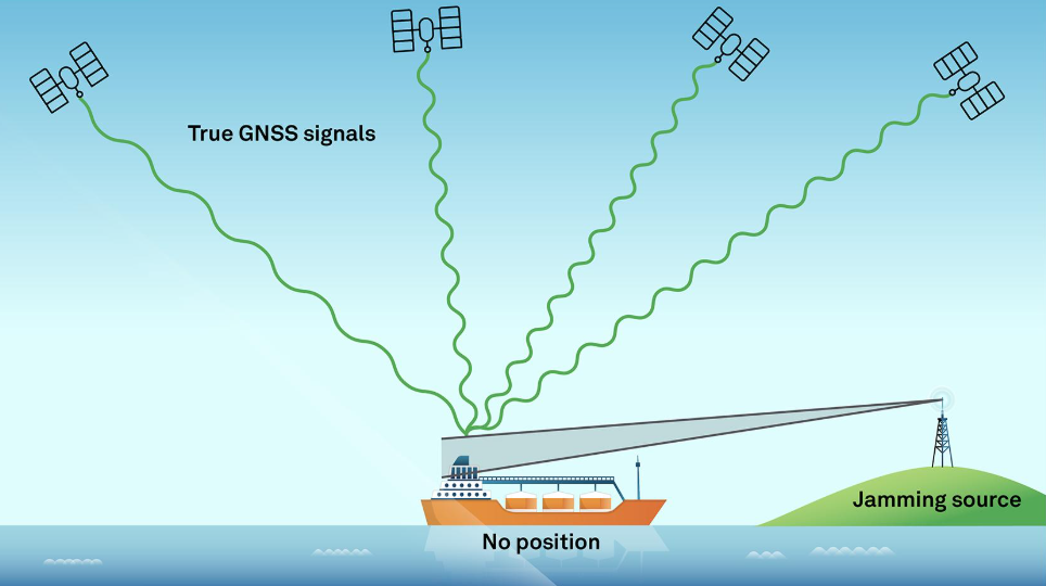
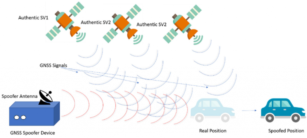
The terms interference, jamming, and spoofing are often used interchangeably, but they represent different engineering problems. Jamming is primarily an availability problem; spoofing is an integrity and trust problem.

Threat	What it does	Typical objective	Primary mitigation
Unintentional interference	Adds unwanted RF signal or raises the noise floor	Degrade GNSS performance	Filtering, dynamic range, interference monitoring
Jamming	Deliberately overwhelms GNSS signals	Deny or degrade availability	Spatial nulling, filtering, robust processing
Spoofing	Transmits counterfeit GNSS-like signals	Mislead the PNT solution	Authentication, consistency checks, sensor fusion

A CRPA is primarily an interference-mitigation technology, not an authentication mechanism. It can improve resilience against some jamming and spoofing scenarios through spatial discrimination, but it does not guarantee that interference will be rejected.

Its effectiveness depends on array geometry, calibration, interference direction, signal environment, and adaptive processing. In some conditions, a CRPA can produce an imperfect null, suppress desired GNSS signals, or even increase the effective gain toward an interferer.

A CRPA provides spatial degrees of freedom; it does not guarantee spatial protection. And while it can reject a signal based on where it comes from, it cannot determine by direction alone whether that signal is authentic.

6. How Many Jammers Can a CRPA Suppress?

This is one of the most misunderstood specifications on an anti-jam datasheet.

A common rule of thumb is that an N-element array provides N−1 spatial degrees of freedom for interference suppression when one constraint is reserved for maintaining the desired GNSS response. This is a useful concept, but it does not mean N−1 jammers can always be perfectly rejected.

For example, a four-element array should not automatically be interpreted as being capable of suppressing three jammers under all conditions. Practical performance depends on array geometry, calibration, frequency, jammer separation, bandwidth, algorithm, dynamic range, and GNSS signal preservation. Closely spaced or broadband interferers, strong near-field sources, calibration errors, and platform scattering can significantly reduce effective suppression.

When evaluating a vendor specification, always ask for the test conditions: frequency and bandwidth, interference waveform and power, number and angular separation of interferers, static or dynamic scenario, and whether the result is measured as null depth at the array output or end-to-end GNSS/PNT performance.

7. Matching Protection to the Application

There is no universal ‘best’ anti-jam antenna. Protection should be sized against three things: the threat, the consequence of losing trustworthy PNT, and the platform’s size/weight/power/cost constraints.

Application	Typical exposure	Practical architecture	Main constraint
Consumer IoT / asset tracking	Low to moderate; mainly unintentional interference	Good FRPA + receiver interference detection	Cost and power
Automotive / fleet telematics	Urban RF congestion, multipath, occasional jamming	High-quality multi-band FRPA + receiver mitigation and monitoring	Cost, integration, packaging
Timing infrastructure	Moderate exposure; very high outage consequence	High-performance antenna + filtering/receiver mitigation; consider CRPA where threat warrants	Availability, long life, holdover
Surveying / RTK / precision agriculture	Moderate; interference can corrupt availability and measurement quality	Multi-band FRPA or CRPA according to site risk + receiver mitigation	Accuracy, cost, field practicality
Maritime	Moderate to high; RF congestion and deliberate interference possible	Pattern-shaped or CRPA depending on threat; robust monitoring	Marine environment, installation
UAV / robotics	Moderate to high; SWaP is critical	Compact CRPA or advanced receiver-level mitigation	Size, weight and power
Defence / assured PNT	High; deliberate and adaptive threats	CRPA + resilient receiver + monitoring + complementary PNT	Mission assurance rather than unit cost

The right choice should be driven by the level of threat and the consequences of losing GNSS. A high-end CRPA can be unnecessary overengineering for a low-value tracker, while a basic FRPA may leave a safety- or mission-critical platform dangerously exposed to deliberate, high-power interference. The antenna architecture should match the threat—not simply the product price or performance headline.

8. Why Monitoring Still Matters When You Have a CRPA

Protection without visibility is incomplete. A GNSS receiver can be significantly degraded before it reports a complete loss of position, and it may continue producing a plausible PVT solution while measurement quality is deteriorating. Useful indicators include:

AGC or RF-level indicators — reveal changes in the interference environment and unexpected increases in received power.
C/N₀ trends — expose loss of signal margin and abnormal degradation across satellites.
Spectrum and interference monitoring — helps distinguish narrowband, broadband, swept, and other RF disturbances.
Jamming/interference flags — provide a simple, machine-readable indication for system-level decision logic.
Integrity and consistency monitoring — essential for detecting conditions where the solution remains available but may no longer be trustworthy, particularly under spoofing.

But detection alone is not enough. Every alarm should trigger a defined response. Depending on the application, the system may switch navigation modes, increase reliance on inertial sensors, reject suspect measurements, change its timing source, alert the operator, or transition to a controlled degraded mode.

A resilient GNSS system does not just detect that something is wrong—it knows what to do next.

9. Testing: Do Not Buy the Number on the Datasheet

Anti-jam performance is highly scenario-dependent. A single quoted ‘dB of suppression’ or ‘number of jammers’ is not enough to compare two systems.

A meaningful evaluation should define the GNSS bands under test, interference waveforms, jammer power, jammer-to-signal ratio, angular geometry, number of simultaneous interferers, polarization, platform dynamics, and success criteria.

Laboratory testing can be conducted through conducted RF paths or over-the-air testing. Conducted testing is useful for receiver and signal-processing development, while radiated/OTA testing is necessary when the antenna array, spatial response, installation, and coupling between elements are part of the performance claim. Keysight’s current CRPA testing guidance also emphasizes the need to reproduce realistic NAVWAR conditions rather than relying on a single simplistic interferer.

For a serious procurement, ask for test evidence—not just marketing terminology. The most useful result is a system-level demonstration showing that the receiver continues to acquire and track authentic GNSS signals and maintains acceptable PNT performance under defined interference conditions.

10. Vendor Landscape: Understand What You Are Actually Buying

The market is easiest to understand when divided into two broad groups: vendors providing CRPA/anti-jam antenna systems, and receiver or chipset vendors implementing interference mitigation inside the GNSS receiver. Some companies operate in both spaces.

Antenna and CRPA system providers EXAMPLES

Vendor / family	Positioning in the market	What to look at
Antcom CRPAs	Dedicated CRPA arrays for assured PNT	Element count, frequency coverage, antenna-electronics compatibility, SWaP
Hexagon \| NovAtel GAJT	Integrated and federated anti-jam systems across land, marine and airborne platforms	Nulling capability, protected bands, form factor, receiver compatibility, direction finding
Calian / Tallysman	GNSS antennas, pattern shaping and CRPA solutions	Filtering, low-SWaP options, element architecture and integration

Receiver and chipset-level resilience EXAMPLES

Vendor / technology	Approach	Best understood as
Septentrio AIM+	Hardware filtering and receiver-side interference monitoring/mitigation	Receiver-level resilience and visibility
u-blox	Receiver architecture and signal-processing techniques for interference resilience across product families	Low-SWaP receiver-side mitigation; capability varies by device
Unicore NebulasIV / JamShield	Integrated multi-frequency anti-jamming and spoofing detection in selected high-precision modules	SoC/module-level resilience
Quectel	GNSS jamming detection features in selected modules; product capabilities vary	Monitoring and module-level detection rather than a universal CRPA replacement

The important comparison is not simply vendor versus vendor. It is architecture versus architecture. A CRPA system with strong spatial suppression can be the right answer for a contested environment; a receiver with strong interference mitigation may be the better answer for a mass-market product; and a high-quality antenna plus filtering and monitoring may be sufficient for a timing installation whose dominant threat is adjacent-band interference.

11. Questions to Ask Before Selecting an Anti-Jam Solution

What is the actual threat: adjacent-band interference, unintentional RF, consumer jamming, deliberate narrowband jamming, broadband jamming, spoofing, or a combination?
What is the consequence of losing GNSS availability—or worse, accepting an incorrect PNT solution?
Which GNSS constellations and frequencies must remain usable during the interference event?
How many simultaneous interferers must the system handle, and under what geometry?
Is the CRPA supplied as an antenna array only, or does it include antenna electronics and null-forming processing?
Is the output compatible with the intended receiver, and what calibration/configuration is required?
What are the actual SWaP and thermal requirements?
How is performance specified: suppression in dB, maximum J/S, tracking threshold, PVT continuity, or another metric?
Were the claims validated with realistic waveforms and multiple interferers, or only with a laboratory CW signal?
What RF-health and integrity indicators are available to the host system?
What happens when interference is detected—alarm only, mitigation, navigation-mode change, or automatic sensor fallback?
What independent PNT sources are available if GNSS becomes unavailable or untrustworthy?

12. Common Anti-Jam Deployment Mistakes

“We installed a CRPA, but the performance did not improve.”

Check the complete signal chain: array, antenna electronics, receiver compatibility, calibration, cabling, firmware, and installation. A CRPA is a system, not simply a different antenna connector.

“The datasheet says three jammers, so we are protected against three jammers.”

Ask for the exact test conditions. Spatial separation, waveform, bandwidth, frequency, power, polarization, and platform effects can materially change performance.

“Our receiver still has a position, so GNSS is fine.”

A valid PVT output does not prove that the measurements are trustworthy. Monitor RF conditions, signal quality, integrity and cross-sensor consistency.

“Anti-jam means anti-spoof.”

It does not. Spatial filtering can help in some spoofing geometries, but authentication and integrity require additional techniques.

“More nulls must always mean a better product.”

Not necessarily. More elements can increase spatial degrees of freedom, but they also affect size, power, calibration complexity, cost, and integration.

“We chose the highest-performance solution.”

The best solution is the one that meets the threat and mission requirement with an appropriate margin—not necessarily the one with the largest array.

13. Frequently Asked Questions

Is a CRPA always better than an FRPA?

No. A CRPA provides a much more powerful spatial interference-mitigation mechanism, but it adds cost, size, power, complexity and integration requirements. For many low- or moderate-threat applications, a high-quality FRPA combined with a resilient receiver and good monitoring is the better engineering solution.

Can a CRPA stop spoofing?

Not by itself. A CRPA can provide spatial discrimination and may reject a spoofer when the spatial geometry is favorable, but spoofing is fundamentally an integrity problem as well as an RF problem. Authentication, signal consistency checks and independent sensors may be required.

How many simultaneous jammers can a CRPA suppress?

A useful first-order concept is approximately one fewer independent null than the number of antenna elements, but practical capability is product- and scenario-dependent. Treat the vendor’s tested performance—not the rule of thumb—as the specification.

Do I need a CRPA if my receiver already has interference mitigation?

Not necessarily. Receiver-side mitigation can be extremely effective against many interference scenarios. A CRPA becomes increasingly valuable when interference is strong, spatially localized, deliberate, multi-source, or capable of overwhelming the receiver front end.

What is the biggest procurement mistake?

Treating the antenna as an isolated component. The correct unit of analysis is the complete PNT chain: antenna, RF front end, receiver, mitigation algorithms, monitoring, installation and fallback sensors.

14. The Takeaway

There is no such thing as a universally ‘best’ anti-jamming antenna. There is only a protection architecture that is appropriate—or inappropriate—for a particular threat and mission.

A conventional FRPA provides a fixed spatial response. Pattern-shaped antennas can reduce susceptibility to interference from particular directions. A CRPA goes further by using multiple antenna elements and adaptive processing to reshape the spatial response in real time, creating nulls toward interference while preserving useful GNSS signals.

But spatial filtering is only one layer. Receiver dynamic range, filtering, interference detection, signal processing, integrity monitoring, inertial sensors, alternative timing sources and operational procedures determine whether a platform actually remains resilient when GNSS is under attack.

The right question is therefore not: ‘Which anti-jam antenna should we buy?’

The right question is: ‘What level of PNT resilience does this application require, what threats must it withstand, and where should that resilience be implemented?’

Sources and Further Reading

Keysight — CRPA Antennas Explained: Choosing and Testing the Best Anti-Jam Solutions for GPS/GNSS Resilience.
Keysight — How to Conduct CRPA Anti-Jam Antenna Testing.
Antcom — CRPAs for Assured Positioning, Navigation and Timing (APNT).
Hexagon | NovAtel — GNSS Anti-jam Antenna Systems (GAJT) and GAJT product documentation.
Calian — Resilient GNSS and Anti-Jamming Solutions; CR7712EXF documentation.
Septentrio — Advanced Interference Monitoring and Mitigation (AIM+).
Unicore — UM980 / NebulasIV / JamShield product documentation.
Quectel — GNSS Jamming Detection Application Note for BG95/BG77/BG600L series.

Editorial note: Product capabilities change over time and vary by model, firmware and configuration. Vendor-specific statements in this guide should therefore be checked against the current product documentation before being used as procurement specifications.

August 26, 2026

Fixed-Base RTK Explained: How a Surveyed Reference Station Delivers Centimeter-Level GNSS Accuracy

A standalone GNSS receiver can typically determine its position to within a few meters under open-sky conditions.

For everyday navigation, this is sufficient: A vehicle following a road, a pedestrian using a map application, or a fitness tracker measuring distance does not require centimeter-level accuracy.

However, a wide range of professional applications operate at a completely different level of precision. In surveying, precision agriculture, construction, and machine control, a few meters of error is not a minor inconvenience — it can mean a boundary marker placed incorrectly, a grading pass that misses its target elevation, or planting rows that overlap instead of aligning cleanly.

So how does GNSS move from meter-level positioning to centimeter-level accuracy?

The answer, for most high-precision deployments, is RTK — Real-Time Kinematic positioning.

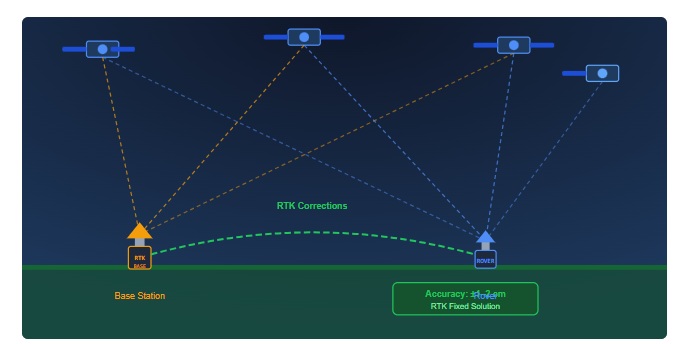
RTK relies on a simple but powerful principle: a second GNSS receiver, installed at a precisely known location, measures many of the same errors affecting the mobile receiver and helps remove them in real time.

Where GNSS errors come from

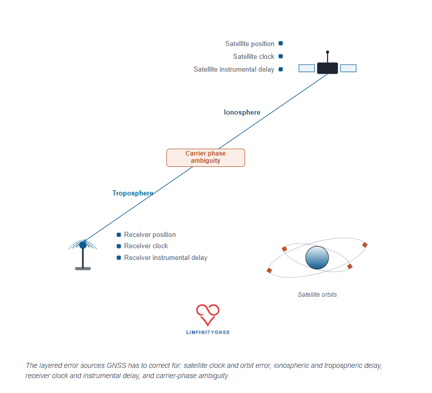
Every GNSS position is calculated from measurements between satellites and the receiver. Those measurements, however, are affected by several distinct error sources:

Satellite clock errors — satellites carry extremely precise clocks, but even a tiny timing error translates directly into a distance error.
Satellite orbit errors — the broadcast position of a satellite is never perfectly accurate.
Ionospheric delay — charged particles in the upper atmosphere slow and distort GNSS signals.
Tropospheric delay — temperature, pressure, and humidity in the lower atmosphere affect signal propagation.
Receiver clock errors — the receiver’s clock is far less precise than the atomic clocks carried onboard satellites.
Receiver hardware delays — antennas, cables and electronics components introduce measurement biases.
Carrier-phase ambiguity — although carrier-phase measurements are extremely precise, the receiver initially does not know the exact number of complete carrier cycles between itself and the satellite.

The challenge is that standalone GNSS positioning has no way to separate and remove these errors on its own. RTK solves this by introducing a second receiver.

The RTK principle: two receivers observing the same errors

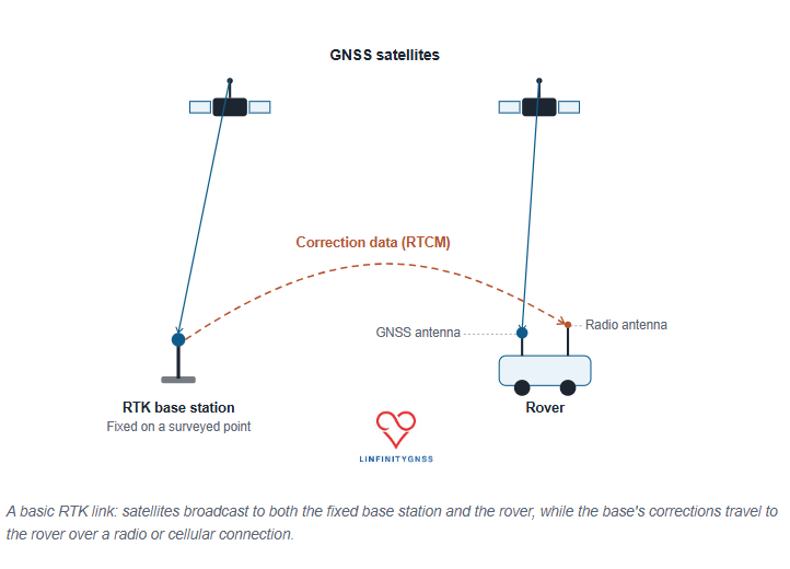
A fixed-base RTK system consists of three components:

A base station installed on a precisely known point.
A rover receiver whose position needs to be determined.
A communication link carrying correction data from the base to the rover.

The key advantage of this system is that the base station already knows exactly where it is — and the rover uses this information by combining its own observations with the base’s through a two-stage process called differencing.

Single Differencing: Eliminating Satellite Errors

The first stage compares observations from the base station and the rover tracking the same satellite at the exact same time.

What it eliminates: Satellite clock errors and satellite instrumental delay. Because these errors originate at the source of transmission, they appear identically in both receivers and cancel out completely when subtracted.
What it reduces: Satellite orbit errors and atmospheric delays (ionospheric and tropospheric). These are heavily mitigated because both receivers look through a similar path in space, though the cancellation becomes less effective as the distance (baseline) between receivers increases.

Double Differencing: Eliminating Receiver Errors

The second stage is called double differencing where the rover’s processing engine selects one satellite as a “pivot” or reference satellite (usually the one highest in the sky with the cleanest signal).It then pairs that reference satellite with every other visible satellite individually.

Receiver clock bias and receiver instrumental delay. Because these errors are due to the receiver’s internal hardware, they affect all satellite observations equally at that moment in time. Comparing two different satellites removes the hardware bias entirely.

What Remains to Be Solved

After this two-stage process, the remaining signal contains only three elements:

The true geometric range difference between the two receivers and the satellites.
A small, residual atmospheric error that grows with baseline length (limiting most RTK setups to a 20 km radius).
The carrier-phase ambiguity, which is the unknown number of full signal wavelengths between the antennas and satellites. Resolving this final integer value is what locks in centimeter-level accuracy.

The effect of differencing can be summarized as follows:

Error Source	Effect of RTK Differencing
Satellite clock error	“Nearly” eliminated
Satellite hardware bias	Eliminated
Receiver clock error	Eliminated
Receiver hardware bias	Eliminated
Orbit error	Strongly reduced
Atmospheric delay	Reduced
Carrier-phase ambiguity	To be resolved

The fixed base station: the foundation of RTK accuracy

A fixed base station is a GNSS receiver installed on a stable point with accurately known coordinates. That coordinate can be obtained one of two ways.

Fixed coordinate mode

The true position of the antenna is already known, from a previous survey or reference measurement, and entered directly into the receiver — usually in Earth-Centered Earth-Fixed (ECEF) coordinates. This is the preferred approach for permanent reference stations.

Survey-in mode

The receiver determines its own position by averaging many GNSS observations over time. A short survey-in period may be sufficient for temporary setups and quick debugging, while a high-quality permanent reference station typically requires a much longer averaging period — often around 12 hours — to arrive at a stable coordinate.

Once the base coordinate is fixed, the receiver continuously compares where it knows it is against where its raw GNSS measurements suggest it is. That difference becomes the correction information sent to the rover.

Why the base antenna matters

The quality of the antenna places a practical ceiling on RTK performance. A “good” reference antenna should provide the following.

Stable installation

The antenna must not move after the coordinate has been calculated. Even a small physical shift introduces error, because the reference point is no longer where the receiver believes it is.

Excellent sky visibility

Obstructions, reflections, and multipath can contaminate measurements. An unobstructed view of the sky in every direction is essential.

Multi-constellation and multi-frequency support

Modern systems commonly track GPS, Galileo, GLONASS, BeiDou, QZSS, and SBAS across multiple frequency bands, which improves robustness and speeds up ambiguity resolution.

Good signal quality

Important antenna characteristics include right-hand circular polarization (RHCP), “suitable gain”, low-noise amplification, and resistance to interference.

The installation environment is also a very important factor — keep it clear of nearby processors, cabling, and other transmitters.

How corrections reach the rover: RTCM and NTRIP

The base station doesn’t transmit a corrected position — it sends measurement information that allows the rover to calculate its own corrected position. The industry-standard format for this information is RTCM (Radio Technical Commission for Maritime Services).

RTCM messages carry:

Pseudorange observations
Carrier-phase measurements
Signal quality indicators
Satellite information
Antenna reference coordinates
Ephemeris information

Modern RTK systems commonly use RTCM 3.x messages, including MSM (Multiple Signal Messages), which support multi-constellation and multi-frequency observations.

A critical practical point: the rover and base must speak the same RTCM language. A mismatch in RTCM version, MSM message type, supported constellations, or correction content is one of the most common reasons for a delayed fix or a failure to ever reach RTK FIX status.

NTRIP: delivering corrections over the internet

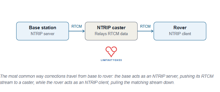
The most common way of distributing RTK corrections today is NTRIP — Networked Transport of RTCM via Internet Protocol. The architecture runs base station → NTRIP server → NTRIP caster → rover.

The base uploads its RTCM correction stream to a caster. The rover connects to that caster as an NTRIP client and requests the appropriate correction stream, usually identified by a mountpoint. This approach allows a single reference station network to support a large number of users without requiring a direct radio connection between base and rover.

The rover: where the final position is calculated

The rover is the moving receiver whose position is actually required. It needs:

A reliable communication link
A suitable GNSS antenna
Compatible correction data
Sufficient satellite visibility

Cellular connectivity, especially LTE, is commonly used for the communication link, since it offers wide coverage and sufficient bandwidth for the correction stream.

The rover continuously evaluates the incoming correction data and attempts to resolve the carrier-phase ambiguities. Its output normally includes a positioning status:

RTK FIX — integer ambiguities successfully resolved; centimeter-level accuracy is achievable.
RTK FLOAT — ambiguity resolution hasn’t completed; accuracy is typically at the decimeter level or worse.

When troubleshooting RTK performance, this status is usually the first thing to check.

The baseline limitation: why distance matters

Fixed-base RTK has a fundamental limitation: the distance between base and rover. The farther apart they are, the less similar their error environment becomes. A rover 5 km from the base observes almost the same atmosphere as the base does. A rover 100 km away does not.

As the baseline increases, atmospheric errors become less correlated, ambiguity resolution becomes harder, and accuracy gradually decreases. A common operational guideline keeps the rover within roughly 20 km of the base for reliable traditional RTK.

For larger coverage areas, correction networks use approaches such as a Virtual Reference Station (VRS). Instead of relying on one distant physical base, the network combines several reference stations and synthesizes a virtual reference point close to the rover — reducing atmospheric differences and improving fix reliability.

Common RTK problems and causes

The receiver stays in FLOAT mode

Common causes: incompatible RTCM messages, insufficient satellite visibility, multipath, poor signal quality, or an excessive baseline distance.

No fix despite an apparently correct configuration

Check the antenna installation, nearby interference sources, correction stream availability, and satellite tracking quality. Carrier-to-noise ratio is an important indicator — poor signal quality can prevent reliable ambiguity resolution even when the rest of the setup looks correct.

Fix degrades during movement

Possible causes: cycle slips, high dynamics, interruptions in the correction stream, or a baseline that’s simply too long.

Frequently asked questions

How many satellites are required for RTK?

The exact requirement depends on the receiver and configuration, but a greater number of satellites across multiple constellations improves reliability. Modern multi-constellation receivers commonly track dozens of signals, providing much stronger redundancy than older single-constellation systems.

Do corrections need to be continuous?

For dynamic applications, continuous correction delivery is essential. Static or slow-moving applications may tolerate short interruptions, but performance depends heavily on receiver design and the surrounding environment.

Does more correction data mean higher cost?

Usually, yes. Higher-density RTCM messages provide more information but require more bandwidth. Reducing the message rate saves data but may reduce robustness, especially for a moving receiver.

The takeaway

Fixed-base RTK remains the foundation of centimeter-level GNSS positioning. The concept itself is simple: a receiver sits on a precisely known point, measures the errors affecting GNSS signals, and sends correction data to another receiver. The rover uses those corrections to resolve carrier-phase ambiguities and determine its position with centimeter-level accuracy.

The technology is mature, but reliable performance depends on getting the details right — antenna quality, reference coordinate accuracy, RTCM compatibility, communication reliability, and baseline distance.

RTK isn’t simply about receiving corrections. It’s about establishing a trustworthy relationship between two receivers — one fixed, one moving — and using that relationship to turn imperfect satellite measurements into precise, dependable positioning.

A standalone GNSS receiver can typically determine its position to within a few meters under open-sky conditions. For everyday navigation, this is sufficient: A vehicle following a road, a pedestrian using a map application, or a fitness tracker measuring distance does not require centimeter-level accuracy. However, a wide range of professional applications operate at a…

July 7, 2026

GNSS Jamming Detection and Spoofing: Why a position fix is not enough?
GNSS jamming and spoofing pose critical risks to positioning systems. Learn why multi-constellation receivers are not enough and what true GNSS integrity and resilience require.

Modern GNSS receivers are highly capable systems. They acquire signals from multiple constellations, track satellites across multiple frequencies, and deliver a position solution with high apparent confidence.

The challenge is that this confidence can be misleading.

A receiver may report a valid position, stable tracking, and strong signal conditions—while the output itself is incorrect.

In many cases, there are:
- No alarms
- No explicit warnings
- No loss of signal
Just a plausible navigation solution derived from corrupted or deceptive inputs.

This is the core issue behind GNSS spoofing and jamming resilience: failure is not always visible.

For organisations relying on positioning, navigation, and timing (PNT), the consequences extend beyond positioning errors into operational, safety, and timing-critical failures.

GNSS Jamming vs Spoofing: Two Fundamentally Different Threats

GNSS interference is often treated as a single problem. In reality, jamming and spoofing represent fundamentally different failure modes requiring different responses.

GNSS Jamming (Signal Denial)

GNSS jamming occurs when radio-frequency interference raises the noise floor, preventing receivers from tracking satellite signals.

Because GNSS signals are extremely weak, even low-power interference can disrupt reception.

Typical effects of jamming:
- Loss of satellite lock
- Reduced carrier-to-noise ratio (C/N₀)
- Position solution degradation or complete loss
- Switch to fallback navigation (if available)
Jamming is usually:
- Sudden
- Detectable
- Associated with signal degradation
Jamming tells you something is wrong.

GNSS Spoofing

Spoofing replaces authentic GNSS signals with counterfeit ones that mimic real satellites.

The receiver continues operating normally.

Typical effects of spoofing:
- Continuous tracking of satellites
- Stable signal metrics
- Valid-looking navigation solution
- No obvious alarms
Spoofing tells you everything is fine—while the output is wrong.

This makes spoofing particularly dangerous for autonomous and safety-critical systems.

Why Multi-Constellation GNSS Is Not Enough

Using multiple GNSS constellations—GPS, Galileo, GLONASS, and BeiDou—can improve availability and provide some resilience against jamming, as interference may not affect all signals equally.

However, multi-constellation capability does not eliminate the risk of spoofing.

A sophisticated attacker can generate counterfeit signals across multiple constellations simultaneously, while maintaining realistic satellite geometry, orbital behaviour, and timing consistency. To the receiver, everything appears normal.

As a result:
- The receiver observes what appears to be a healthy satellite sky.
- Signal quality metrics remain within expected limits.
- The navigation solution is calculated with high confidence.
- There is no obvious indication that the position is being manipulated.
Multi-frequency and multi-constellation processing can help detect poorly executed or inconsistent spoofing attempts. However, well-designed attacks can remain undetected unless additional integrity monitoring and signal authentication mechanisms are in place.

The key lesson is simple: more satellites do not automatically mean more trust. True GNSS resilience requires independent validation of the navigation solution, not just additional signals.

Conclusion: Multi-constellation capability is necessary, but not sufficient for GNSS resilience.

GNSS Integrity Monitoring: The Real Challenge

GNSS integrity is the ability to assess whether a navigation solution is reliable and trustworthy.

The fundamental challenge is not whether a position is available—it is whether that position is correct.

Most GNSS systems are designed to optimise for:
- Continuous signal tracking
- Consistent navigation output
- Maximum position availability
However, they are often not designed to:
- Detect deliberate deception
- Identify and classify interference events
- Recognise when a seemingly valid position is actually wrong
- Reject plausible but manipulated navigation solutions
This creates what is known as the integrity gap.

A jammed receiver often loses signals and raises alarms. A spoofed receiver, by contrast, may continue operating normally while reporting a false position with complete confidence. Even partial degradation can remain undetected if it does not exceed predefined alert thresholds.

In other words, the most dangerous GNSS failures are not always the ones that stop navigation—they are the ones that quietly provide the wrong answer.

Five Layers of GNSS Resilience

True resilience requires layered architecture—not a single feature.

1. Cryptographic Authentication (Galileo OS-NMA)

The European GNSS Agency introduced Galileo OS-NMA (Navigation Message Authentication) in 2025.

It allows receivers to verify navigation message authenticity.

Limitations:
- Only applies to Galileo E1 signals
- No equivalent full civilian GPS authentication yet
When available, OS-NMA should be enabled and properly integrated.

2. Inertial Fusion (IMU Integration)

GNSS can be manipulated. Physics cannot.

IMUs provide independent motion data.

Benefits:
- Detect GNSS vs motion inconsistencies
- Identify spoofing-induced drift
- Provide continuity during outages
Architectures:
- Loosely coupled → basic detection
- Tightly coupled → high resilience
- Deep integration → strongest protection
Tight coupling is recommended for safety-critical systems.

3. Signal-Level Detection

Traditional methods rely on:
- C/N₀
- AGC
- Residual errors
These are increasingly insufficient.

Modern systems use:
- Time-series anomaly detection
- RF behaviour modelling
- Machine learning classification
Key principle: detection is stronger at signal-processing level than after position computation.

4. Independent PNT Sources

No GNSS system is fully resilient on its own.

Alternative PNT sources include:
- eLoran (terrestrial navigation and timing)
- 5G Advanced positioning
- Chip-scale atomic clocks (timing holdover)
Principle: Critical systems must never rely on a single PNT source.

5. Human Factors and Operational Awareness

Technology alone does not ensure resilience.

Operators must understand:
- Jamming = signal loss or degradation
- Spoofing = correct-looking but false data
Required responses:
- Jamming → fallback navigation
- Spoofing → reject data integrity
Most dangerous failure mode is not GNSS loss—it is trusting incorrect GNSS data.

Five Questions to Ask Your GNSS Vendor

Before selecting a receiver or system:
1. Does it support Galileo OS-NMA and how is it implemented?
2. Where does spoofing detection occur (signal or solution level)?
3. What level of IMU coupling is used?
4. What independent PNT sources are supported?
5. How are jamming and spoofing differentiated in alerts?
If answers are unclear, system maturity is likely limited.

The Future of GNSS Resilience

GNSS interference is not a temporary issue—it is an evolving operational reality.

Future resilience will depend on integration of:
- Authentication
- Sensor fusion
- Signal analytics
- Multi-source PNT
- Operational training
Multi-constellation receivers are a foundation—but not a complete solution.

Conclusion

GNSS jamming and spoofing represent fundamentally different threats.
- Jamming is visible and disruptive
- Spoofing is silent and deceptive
The real challenge is not maintaining signal reception—it is maintaining trust in the navigation solution.

True GNSS resilience requires system-level architecture, not receiver-level assumptions.

The future of GNSS resilience will not be defined by how many satellites a receiver can track.

It will be defined by how confidently it can determine whether those signals should be trusted.

Because the most dangerous GNSS failure is not losing position.

It is acting on a position that is wrong.

.
GNSS jamming and spoofing pose critical risks to positioning systems. Learn why multi-constellation receivers are not enough and what true GNSS integrity and resilience require. Modern GNSS receivers are highly capable systems. They acquire signals from multiple constellations, track satellites across multiple frequencies, and deliver a position solution with high apparent confidence. The challenge is…

June 22, 2026
AI in GNSS
AI in GNSS: Why Cybersecurity Can’t Be an Afterthought

Written by

LinfinityGNSS in GNSS Technical Articles

AI in GNSS: Why Cybersecurity Can’t Be an Afterthought

AI is rapidly becoming embedded in GNSS systems — from signal processing and anti-jam/anti-spoof detection through to autonomous positioning corrections. For most teams, the conversation about AI has so far focused on accuracy, data quality, and regulatory compliance.

That’s an incomplete picture.

AI is not just a data problem or a compliance problem. It is a security problem — and for GNSS-dependent navigation, timing, and infrastructure systems, getting this wrong has consequences that go well beyond a failed audit.

Here’s what every GNSS engineering team needs to understand.

1. Cybersecurity Is a Precondition, Not an Add-On

The Guidelines for Secure AI System Development (2023) state it plainly:

“Cybersecurity is a necessary precondition for the safety, resilience, privacy, fairness, efficacy and reliability of AI systems.”

This is easy to read past, but it’s worth sitting with. It doesn’t say cybersecurity is one of several important properties. It says the other properties — safety, fairness, reliability — depend on it. An AI system that isn’t secure cannot meaningfully be called safe or reliable, no matter how good its outputs look in testing.

Why this matters for GNSS A positioning or timing system that performs beautifully on the bench but rests on an insecure AI component isn’t a robust system — it’s a system with an unverified dependency.

2. What “High-Risk” Actually Requires

For systems classified as high-risk — and GNSS-dependent navigation, timing, and critical infrastructure squarely fall into this category — the bar is set across several dimensions simultaneously:
- Accuracy — the model performs to the standard the application demands
- Robustness — performance holds up under degraded, noisy, or adversarial conditions
- Cybersecurity — the model and its data pipeline resist manipulation
- Risk management — failure modes are identified and mitigated, not just documented
- Data governance — training and operational data is controlled, traceable, and clean
- Human oversight — a person remains meaningfully in the loop
Fix None of these can be treated as a separate workstream ticked off independently. A model can be highly accurate and still be insecure; it can be secure and still lack proper oversight. Build your assurance case so these properties are demonstrated together, not in isolation.

3. The Threat Surface Has Moved Inside the Model

This is the shift that catches many teams out.

Historically, securing a GNSS system meant securing the hardware, the RF front end, and the network around it. With AI in the loop, the model itself becomes part of the attack surface.

Consider an AI system trained to detect spoofing or jamming on a GNSS signal. If that model can be subtly poisoned, manipulated, or degraded, it doesn’t just stop working — it can continue to appear to work while quietly failing. A compromised model could mask the very interference it was built to flag, giving operators false confidence at exactly the moment accurate information matters most.

This mirrors a problem GNSS engineers already know well from spoofing: the most dangerous failures are the ones that don’t trigger an alarm.

Fix Treat the AI model with the same scrutiny you’d apply to a GNSS signal chain. Monitor for drift, unexpected confidence patterns, and outputs that don’t align with independent sensor data (e.g. IMU). If your spoofing-detection AI starts behaving “too well,” that’s worth investigating, not celebrating.

4. Build Security In From the Start

Retrofitting security after an AI system is deployed is significantly harder — and significantly riskier — than designing it in from the outset. In practice, this means:
- Treating model integrity with the same rigour as data quality and algorithmic fairness — it’s not a lesser concern, it’s part of the same assurance picture
- Defining clear acceptance criteria for AI outputs, so that every decision in the loop has a documented threshold for what counts as a valid, trustworthy result — not just “the model said so”
- Involving security expertise during system design, not only during late-stage testing
- Building incident response plans that account for AI-specific failure modes, including subtle manipulation that may not trigger traditional alerts
Fix Ask, early in your design process: if this model were quietly wrong, how would we know? If you don’t have a confident answer, your acceptance criteria and monitoring strategy need work before deployment — not after.

5. Securing the Intelligence Layer

As GNSS systems become smarter, more adaptive, and more autonomous, security has to evolve with them. Securing the signal is no longer enough — securing the intelligence layer (the models, the data pipelines, the decision logic sitting on top of the signal) is now just as critical.

For organisations operating in this space, the takeaway is simple: bring cybersecurity thinking into AI design early, treat AI security as inseparable from AI safety, and recognise that the next generation of GNSS resilience depends as much on protecting the algorithms as it does on protecting the antennas.

The Bottom Line

AI brings real capability to GNSS — better spoofing detection, smarter signal processing, more autonomous correction. But every one of those capabilities depends on the AI component itself being secure, monitored, and held to clear acceptance criteria.

If you’re integrating AI into a GNSS-dependent system and want a second opinion on your security and assurance approach, we’re happy to take a look.
AI in GNSS: Why Cybersecurity Can’t Be an Afterthought Written by LinfinityGNSS in GNSS Technical Articles AI in GNSS: Why Cybersecurity Can’t Be an Afterthought AI is rapidly becoming embedded in GNSS systems — from signal processing and anti-jam/anti-spoof detection through to autonomous positioning corrections. For most teams, the conversation about AI has so far…

June 19, 2026

GNSS Correction Services Explained

GNSS Correction Services Explained: From RTK to PPP-RTK

Global Navigation Satellite Systems (GNSS), including GPS, Galileo, GLONASS, and BeiDou, underpin a rapidly growing ecosystem of applications ranging from precision agriculture and surveying to autonomous systems, robotics, and connected mobility.

While standalone GNSS positioning enables global navigation with metre-level accuracy, many modern applications require significantly higher performance.

Achieving decimetre- or centimetre-level positioning requires the mitigation of multiple error sources that affect GNSS measurements. This is the role of GNSS correction services.

Understanding the capabilities, limitations, and underlying principles of these services is essential for selecting the most appropriate solution for a given application.

Why Are GNSS Corrections Required?

A standalone GNSS receiver determines its position by estimating the distance, or pseudorange, to multiple satellites. The resulting position solution is affected by several error sources, including:

Satellite clock errors
Satellite orbit errors
Ionospheric and tropospheric delays
Multipath
Receiver noise

Collectively, these errors limit standard positioning performance to approximately 3–10 metres, depending on receiver quality, environmental conditions, and satellite geometry.

GNSS correction services improve positioning performance by estimating and compensating for these errors using measurements from reference stations with precisely known coordinates.

Depending on the correction methodology employed, positioning accuracy can be improved from metre-level to centimetre-level performance.

How Do GNSS Correction Services Work?

A reference station continuously receives signals from GNSS satellites and calculates the errors affecting those signals.

These corrections are then delivered to a user’s GNSS receiver, commonly referred to as a rover. The rover applies the corrections to improve its position estimate.

Corrections can be delivered through various communication channels, including:

NTRIP over internet connections
UHF or VHF radio links
L-band satellite services
Direct satellite broadcasts

It is important to distinguish between the correction method and the delivery method. For example, RTK is a positioning technique, while NTRIP is a protocol used to transmit correction data over the internet.

Observation Space Representation (OSR) and State Space Representation (SSR)

GNSS correction services are generally based on one of two approaches.

Observation Space Representation (OSR)

OSR corrections are generated for a specific user location and applied directly to GNSS observations.

Traditional RTK and Network RTK services use OSR corrections.

OSR approaches provide rapid ambiguity resolution and excellent positioning performance but require dense reference station networks and generate user-specific correction streams.

State Space Representation (SSR)

SSR corrections model individual error sources, including:

Satellite orbit errors
Satellite clock errors
Signal biases
Atmospheric delays

SSR corrections are independent of user location, making them more scalable for large numbers of users.

PPP and PPP-RTK services typically use SSR corrections.

Satellite-Based Augmentation Systems (SBAS)

Satellite-Based Augmentation Systems provide wide-area corrections generated from regional reference networks and broadcast through geostationary satellites.

Examples include:

EGNOS in Europe
WAAS in North America
MSAS in Japan
GAGAN in India

SBAS services primarily compensate for satellite orbit, clock, and ionospheric errors, improving standalone positioning accuracy to approximately 0.5–2 metres.

SBAS also provides integrity information, making it particularly valuable for aviation applications.

Differential GNSS (DGNSS)

Differential GNSS uses code-based corrections generated by a nearby reference station.

Because many GNSS errors are spatially correlated, users operating within a limited distance of the reference station can benefit from significant improvements in positioning accuracy.

DGNSS typically delivers sub-metre performance and remains widely used in marine navigation, GIS mapping, and asset management applications.

Real-Time Kinematic (RTK)

Real-Time Kinematic positioning uses carrier-phase measurements from a local reference station or network of reference stations to achieve centimetre-level accuracy.

RTK performance depends on resolving carrier-phase ambiguities as integer values.

Once ambiguities are fixed, RTK can achieve horizontal accuracies of 1–3 cm and vertical accuracies of 2–5 cm within seconds.

However, RTK performance is constrained by baseline length because atmospheric errors become less correlated as the distance between the rover and the reference station increases.

Single-base RTK is typically limited to baselines of approximately 10–20 km.

Network RTK addresses this limitation by modelling atmospheric errors across a network of Continuously Operating Reference Stations (CORS), enabling high-accuracy positioning over larger regions.

Common Network RTK implementations include:

Virtual Reference Station (VRS)
Master Auxiliary Concept (MAC)
Flächen-Korrektur-Parameter (FKP)

RTK is widely used in:

Land surveying
Construction and machine control
Precision agriculture
UAV mapping
Mining operations

Precise Point Positioning (PPP)

Precise Point Positioning achieves high-accuracy positioning without requiring local reference stations.

Instead, PPP relies on precise satellite orbit, clock, and bias information generated from global reference networks.

Unlike RTK, PPP offers global coverage and is particularly well suited to applications operating in remote areas.

Modern multi-frequency PPP solutions can achieve decimetre- to centimetre-level accuracy. However, convergence remains a key limitation.

Depending on receiver capabilities, correction quality, and environmental conditions, convergence times typically range from 10 to 40 minutes.

PPP is commonly used for:

Offshore and maritime operations
Remote monitoring
Scientific applications
Large-scale infrastructure monitoring

PPP-RTK

PPP-RTK combines the scalability of PPP with the rapid convergence characteristics of RTK.

In addition to precise satellite products, PPP-RTK services provide atmospheric corrections and phase bias information that enable rapid ambiguity resolution.

By reducing convergence times from tens of minutes to seconds or a few minutes, PPP-RTK addresses one of the primary limitations of traditional PPP.

PPP-RTK is increasingly viewed as the enabling technology for high-volume, high-precision applications, including:

Autonomous vehicles
Robotics
Connected mobility
Uncrewed aerial systems (UAS)
Mass-market high-precision positioning

Performance Comparison

Correction Service	Typical Accuracy	Coverage	Convergence Time	Infrastructure Requirement
Standalone GNSS	3–10 m	Global	Immediate	None
SBAS	0.5–2 m	Regional	Immediate	None
DGNSS	0.3–1 m	Local to regional	Seconds	Reference station
RTK	1–3 cm	Local	Seconds	Local base station
Network RTK	1–3 cm	Regional	Seconds	CORS network
PPP	5–20 cm	Global	10–40 minutes	Global correction service
PPP-RTK	2–5 cm	Regional to global	Seconds to minutes	SSR correction service

How to Select the Right Correction Service

Selecting the appropriate correction service depends on several factors:

Required accuracy
Coverage area
Convergence time requirements
Availability of communication infrastructure
Scalability requirements
Cost

As a general guideline:

Navigation applications typically use SBAS.
Mapping and GIS applications often use DGNSS.
Surveying, construction, and machine control applications rely on RTK or Network RTK.
Remote operations without local infrastructure benefit from PPP.
High-volume autonomous and robotic applications increasingly adopt PPP-RTK.

Challenges and Limitations

Regardless of the correction service employed, positioning performance remains sensitive to environmental conditions.

Key challenges include:

Multipath and signal obstruction
Limited sky visibility
GNSS interference, jamming, and spoofing
Communication outages
Poor antenna installation

Even the most advanced correction service cannot compensate for severely degraded signal conditions.

Reliable high-accuracy positioning requires careful consideration of the receiver, antenna, correction service, and communication infrastructure.

Conclusion

GNSS correction services have evolved significantly from traditional differential techniques to globally scalable SSR-based solutions.

RTK remains the benchmark for rapid centimetre-level positioning in localised applications, while PPP enables high-accuracy positioning in areas without supporting infrastructure.

PPP-RTK is emerging as the next-generation architecture for scalable, high-precision positioning, bridging the gap between global coverage and rapid convergence.

As demand grows for autonomous systems, connected mobility, and intelligent infrastructure, understanding the strengths and limitations of each correction approach is becoming increasingly important for engineers, system architects, and technology decision-makers.

GNSS Correction Services Explained: From RTK to PPP-RTK Global Navigation Satellite Systems (GNSS), including GPS, Galileo, GLONASS, and BeiDou, underpin a rapidly growing ecosystem of applications ranging from precision agriculture and surveying to autonomous systems, robotics, and connected mobility. While standalone GNSS positioning enables global navigation with metre-level accuracy, many modern applications require significantly higher…

June 16, 2026

Choosing the Right GNSS Module for Your Application

In today’s rapidly evolving industrial landscape, connectivity plays a critical role in driving efficiency, productivity, and operational visibility. From asset tracking and fleet management to autonomous systems and precision agriculture, accurate positioning data is essential for informed decision-making and streamlined operations.

At the heart of these solutions is the Global Navigation Satellite System (GNSS) module — a technology that enables reliable and precise location tracking. However, with a wide range of GNSS module options available, selecting the most suitable solution for your application can be challenging.

This guide explores the key GNSS module categories, outlines the factors to consider when selecting a GNSS solution, and highlights the ideal use cases for each technology.

Understanding Your Application Requirements

Before selecting a GNSS module, it is important to evaluate your operational requirements. Several factors will influence the most appropriate solution.

Accuracy Requirements

The level of positioning accuracy required is often the most important consideration. Standard navigation and tracking applications typically require metre-level accuracy. Surveying, autonomous navigation, precision agriculture, and machine control applications often require centimetre-level positioning, achievable using Real-Time Kinematic (RTK) technology.

Operating Environment

The environment in which the GNSS module operates directly impacts performance. Open-sky environments generally allow standard GNSS modules to perform effectively. Urban canyons, dense forests, tunnels, and underground parking structures can obstruct satellite signals, requiring enhanced technologies such as dead reckoning or multi-frequency GNSS.

Frequency Band Requirements

GNSS modules are available in single-band and multi-band configurations. Single-band modules are suitable for most standard positioning applications. Dual-band or multi-band modules provide improved signal reliability, faster RTK convergence, and enhanced performance in challenging environments.

Power Consumption

Power requirements should be considered particularly for battery-powered devices and remote monitoring systems where energy efficiency is critical.

Positioning Continuity

Applications that must maintain accurate positioning during temporary GNSS signal loss should incorporate dead reckoning capabilities through integrated inertial sensors.

The Three GNSS Module Categories

Standalone GNSS

Metre-level accuracy. Ideal for tracking, IoT, and standard navigation. Low power, cost-effective.

🚗

Dead Reckoning

Continuous positioning via IMU during signal outages. Essential for urban and tunnel environments.

🎯

High-Precision RTK

Centimetre-level accuracy. Required for surveying, autonomous vehicles, and precision agriculture.

Standalone GNSS Modules

A typical GNSS receiver module with multi-constellation support

Standalone GNSS modules are ideal for applications that require accurate positioning without additional communication or sensor integration. These modules feature an integrated GNSS receiver and antenna, enabling them to independently acquire and process satellite signals.

Typical Applications

Asset tracking and monitoring
Personal navigation devices
Location-based services
Basic telematics systems
IoT positioning applications

Key Benefits

Cost-effective implementation
Low power consumption
Fast Time-to-First-Fix (TTFF)
Support for GPS, Galileo, GLONASS, and BeiDou
Reliable metre-level positioning accuracy

Standalone GNSS modules deliver dependable positioning performance for a wide range of industrial and commercial applications where standard navigation accuracy is sufficient.

Dead Reckoning GNSS Modules

Dead reckoning uses onboard IMU sensors to maintain positioning continuity through tunnels and urban canyons

In environments where satellite signals may be obstructed or temporarily unavailable, dead reckoning GNSS modules provide enhanced positioning continuity. These solutions combine GNSS technology with inertial measurement sensors (IMUs) to estimate and maintain position during periods of signal degradation or loss.

Typical Applications

Fleet management
Vehicle telematics
Urban navigation systems
Logistics and delivery vehicles
Connected automotive systems

Ideal Environments

Urban canyons
Tunnels and underground parking facilities
Dense forests and foliage
Industrial facilities with intermittent GNSS coverage

Key Benefits

Continuous positioning during signal outages
Improved navigation reliability
Enhanced route accuracy in dense urban environments
Seamless transition between GNSS and inertial navigation

Dead reckoning GNSS modules ensure consistent and dependable location tracking, making them particularly valuable for applications that require uninterrupted positioning data.

High-Precision GNSS Modules

RTK positioning uses corrections broadcast from a base station to achieve centimetre-level accuracy at the rover

For applications where positioning accuracy is mission-critical, high-precision GNSS modules offer advanced capabilities and exceptional performance. Leveraging Real-Time Kinematic (RTK) positioning, these modules can achieve centimetre-level accuracy in real time.

Typical Applications

Land surveying and mapping
Precision agriculture
Construction and machine control
Autonomous vehicles and robotics
Infrastructure monitoring
Unmanned aerial vehicles (UAVs)

Key Benefits

Centimetre-level positioning accuracy
Multi-frequency GNSS support
Faster RTK convergence times
Improved performance in challenging environments
Enhanced reliability for mission-critical operations

High-precision GNSS systems typically require correction data from an RTK base station or NTRIP correction service to achieve their highest levels of accuracy.

Matching GNSS Technology to Your Application

Use Case	Recommended Module	Accuracy	Key Feature
Asset tracking / IoT	Standalone GNSS	Metre-level	Low power, low cost
Fleet & vehicle telematics	Dead Reckoning	Metre-level	IMU continuity
Urban navigation	Dead Reckoning	Metre-level	Signal gap bridging
Surveying & mapping	High-Precision RTK	Centimetre-level	RTK fixed solution
Precision agriculture	High-Precision RTK	Centimetre-level	Multi-frequency
Autonomous vehicles	High-Precision RTK	Centimetre-level	Fast convergence
UAVs / robotics	High-Precision RTK	Centimetre-level	Heading initialisation

Additional Integration Considerations

Antenna Selection

High-precision applications typically require active, high-performance GNSS antennas to maximise signal quality and positioning accuracy.

Time-to-First-Fix (TTFF)

Applications requiring rapid startup should prioritise modules with fast acquisition performance, Real-Time Clock (RTC) backup, and Assisted GNSS (A-GNSS) support.

Multi-Constellation Support

Modern GNSS modules that support multiple satellite constellations — GPS, Galileo, GLONASS, BeiDou — provide improved availability, reliability, and positioning accuracy across diverse operating environments.

The Bottom Line

Selecting the right GNSS module is a critical step in building a reliable and effective positioning solution. Whether your application requires basic tracking, uninterrupted navigation in challenging environments, or ultra-precise location data, the right technology choice directly impacts operational outcomes.

Choose a Standalone GNSS Modulefor standard positioning and tracking applications.
Choose a Dead Reckoning GNSS Modulewhen continuous positioning is needed in areas with frequent signal interruptions.
Choose a High-Precision RTK GNSS Modulewhen centimetre-level accuracy is essential for operational success.

By carefully evaluating accuracy requirements, operating environment, frequency band, power consumption, and continuity needs, organisations can choose a GNSS solution that delivers optimal performance and long-term value.

If you are unsure which GNSS technology best fits your application, consulting with a GNSS specialist can help identify the ideal solution for your specific operational requirements.

Talk to a GNSS expert →Or email us: info@linfinityGNSS.com

Linfinity GNSS is a Cambridge-based team of precision positioning engineers with 20+ years of hands-on GNSS integration and testing experience. We work with organisations across maritime, defence, automotive, and autonomous systems.

June 16, 2026

AI-Powered GNSS Test Automation: The Future of Field Testing

GNSS Technical Articles

By LinfinityGNSS·8 June 2026·9 min read

Field testing GNSS firmware used to mean weeks of manual driving routes, spreadsheet analysis, and expert sign-off on gut instinct. The scale of modern GNSS product development — multiple product families, growing firmware complexity, and customers demanding granular pass/fail evidence — has made that model untenable.

At LinfinityGNSS Ltd, we’re building a different approach: an intelligent, automated testing framework that combines real-world RF capture, repeatable lab replay, and AI-driven analysis to ensure every firmware release meets the quality bar our customers expect — before it ever reaches them.

This article covers how we think about GNSS testing at scale, how the automated system works, and — critically — where AI is already improving the process and where it will transform it next.

Why GNSS Testing Is So Hard to Scale

Modern GNSS positioning products are no longer simple receivers. They power autonomous vehicles, precision agriculture, maritime navigation, drones, and consumer wearables — each with different performance requirements and dramatically different operating environments.

Testing a firmware release properly means covering:

Field testing — urban, dense urban, highway, tunnel exit, sport scenarios (swimming, running), technology-specific environments (drones, lawnmowers), and pedestrian use cases
System validation — full SW/HW regression, safety-critical standards compliance, and release gating
Hardware testing — module-level checks, reliability (jamming, spoofing), MTBF, stress, and production quality

Four forces are making this harder with every release cycle:

Log complexity: different log formats per product, and a very high number of products
Customer expectations: increasingly granular pass/fail documentation required by both internal and external stakeholders
Release velocity: the volume of tests associated with each validation cycle continues to grow
Analysis depth: manual log review cannot scale — automated parsing and structured output is now a requirement, not a nice-to-have

The Record & Replay Foundation

The centrepiece of our field testing methodology is the Spirent GSS6450 RF Record & Playback System. It captures real-world GNSS, cellular, and wireless RF signals in the field — including RTK corrections and Dead Reckoning data — and reproduces them with full fidelity in the laboratory.

This changes the economics and repeatability of firmware validation. Instead of re-driving test routes every time a new build is ready, teams replay a curated library of gold-standard recordings against every firmware version. The signal environment is identical. The comparison is objective. The result is true repeatability at scale.

Key benefits:

Capture data across diverse geographies — not just one region — to ensure algorithms perform reliably worldwide
Train positioning algorithms with real RTCM corrections and replay the data as many times as needed
Enable genuine benchmarking between different firmware versions, hardware variants, and competing products
Re-collect logs from the field if a new edge case is discovered, without repeating the entire test campaign

AI Enhancement

LLM-based classifiers can be applied at ingestion time to automatically tag and categorise recorded scenarios — classifying signal complexity, environment type, multipath severity, and likely failure modes. This allows the system to prioritise the most diagnostically valuable replays in regression runs, rather than running everything every time.

The Automated Testing System — How It Works

The automated testing platform is built around a self-service web interface. From a browser, a user selects the configuration — module type, firmware version, hardware variant, test scenario — and the system handles everything else.

The workflow is as follows:

Step 1 — Configure. Select module type, firmware version, hardware configuration, and test scenario from the web dashboard.

Step 2 — Orchestrate. The system automatically fetches the replay file and configuration from the central database, then communicates with the GSS6450 to begin the RF replay.

Step 3 — Analyse. Logs are automatically ingested and parsed against KPI thresholds the moment the replay completes.

Step 4 — Report. A structured, colour-coded pass/fail report is generated and delivered by email — no manual intervention required.

AI Enhancement

AI agents embedded in the orchestration layer can dynamically select the most relevant test scenarios for a given firmware diff — analysing the code changes and recommending targeted regression coverage rather than running the full suite every time. This can reduce test cycle time by 40–60% without reducing defect detection sensitivity.

Reporting: Beyond Pass/Fail

Test reports are not simple binary summaries. They are structured intelligence documents covering multiple DUTs (Devices Under Test) across different firmware, hardware, and configuration variants, with truth data from the original field collection as the immutable reference baseline.

Reports include both common KPIs — applied universally across all products — and differentiated KPIs, which are specifically designed for each test scenario and product family. Results are colour-coded:

Result	Colour	Meaning
PASS	Green	Result within acceptable limits for this KPI
LIMIT	Orange	Result near boundary — warrants close review before sign-off
FAIL	Red	Result outside acceptable limits — blocks release or requires root cause

AI Enhancement

Natural language generation models can transform raw KPI data into plain-English failure narratives — automatically explaining why a test failed, which signal conditions contributed, and which firmware components are likely implicated. Engineers spend their time on root cause and fixes, not interpreting data tables.

Where AI Takes This Further

The platform described above is a strong foundation. What follows is the AI-driven roadmap that will define the next generation of GNSS quality assurance.

Predictive failure detection via ML on log history

Train anomaly-detection models on the growing historical log database to identify subtle signal patterns that precede known failure modes — surfacing regression risks before they manifest as customer complaints. The model improves with every release cycle, building institutional memory that no human team could maintain alone.

AI-augmented distributed testing

Expand field coverage by engaging FAE teams and volunteers across global locations to contribute real-world recordings on a regular basis. An AI routing layer automatically classifies incoming data, detects duplicates, and prioritises novel signal environments — ensuring the test corpus grows in quality, not just volume.

Intelligent regression scope optimisation

Apply LLM-based code analysis to each firmware diff to automatically recommend a targeted regression test plan, covering the most likely impact areas without running the full suite. This compresses release cycles without compromising coverage, making continuous delivery viable even for safety-relevant products.

Conversational test intelligence

Embed a conversational AI interface into the reporting platform — allowing engineers, FAEs, and product managers to query test results in plain language. “Which firmware version had the worst urban tunnel re-acquisition performance in the last three releases?” becomes a one-sentence question, not a three-hour data archaeology exercise.

Generative scenario synthesis

Use generative models to synthesise novel, edge-case RF scenarios that are statistically rare in real-world collections but known to stress positioning algorithms — automatically expanding test coverage into corners of the signal space that field teams would never encounter organically.

Stakeholder Reporting Flow

Technology alone is not enough. Test outcomes must reach the right people in the right form. The reporting workflow is structured as follows:

New feature testing — conducted by the ST Team with focused analysis on the integrated feature
Regression testing — a predefined set of tests per product, evolving alongside the product itself
Report review — the ST Team analyses failures and provides context before sharing outward
Distribution — reports shared with FAE, R&D, and PDM teams, the stakeholders closest to customer requirements

This flow ensures test results are actionable — not a data dump, but a curated, decision-ready briefing for each audience.

The Bottom Line

The combination of real-world RF record & replay, web-based test orchestration, automated KPI reporting, and AI-driven intelligence represents a genuine step-change in what GNSS quality assurance can achieve.

Every release cycle is a learning opportunity. Organisations that build systems to capture and act on that learning — making the test infrastructure smarter with every run — will out-quality their competitors permanently. At LinfinityGNSS Ltd, that is exactly what we are building.

If you are planning a GNSS validation programme, scaling a test team, or want to understand how AI can improve your existing testing process, we’re happy to discuss it.

Talk to a GNSS testing expert — whether it’s reviewing your test strategy, helping design KPI frameworks, or integrating record & replay into your workflow, we’re here to help.Consult an expert →Or email us: info@linfinityGNSS.com

Silvana Capasso worked as GNSS test engineer at Intel for >10 years and now she is the co-founder of LinfinityGNSS Ltd, a Cambridge-based team of precision positioning engineers with 20+ years of hands-on GNSS integration and testing experience. We work with organisations across automotive, maritime, and autonomous systems.

GNSS Technical Articles By LinfinityGNSS·8 June 2026·9 min read Field testing GNSS firmware used to mean weeks of manual driving routes, spreadsheet analysis, and expert sign-off on gut instinct. The scale of modern GNSS product development — multiple product families, growing firmware complexity, and customers demanding granular pass/fail evidence — has made that model untenable.…

June 8, 2026

Tag: base

1. Introduction

2. What is multipath?

2.1 Effects on code and carrier-phase measurements

2.2 Factors that influence multipath severity

3. Direct and reflected signal paths

4. How antenna design can reduce multipath

5. Antenna types: practical comparison

6. Selection and installation

6.1 What to check in the datasheet

6.2 Installation practice

7. A practical selection workflow

8. Conclusion

Technical references and further reading

1. Introduction

2. What is a GNSS orbit?

2.1 Describing a GNSS orbit

3. The main orbit families

3.1 Low Earth orbit (LEO)

3.2 Medium Earth orbit (MEO)

3.3 Geostationary orbit (GEO)

3.4 Inclined geosynchronous orbit (IGSO)

3.5 Polar and Sun-synchronous orbits (SSO)

3.6 Orbit comparison at a glance

4. GNSS constellations

4.1 GPS (United States)

4.2 Galileo (European Union)

4.3 GLONASS (Russia)

4.4 BeiDou (China)

4.5 Regional systems

4.6 Constellation comparison

5. Satellite-based augmentation systems (SBAS)

6. Why this matters for GNSS users

Acquisition, Tracking, and Reacquisition

Why Reacquisition Happens So Often

Where the Power Actually Goes

Duty-Cycling Smarter, Not Just Less

Other Levers Worth Engineering For

The Takeaway

1. Standard Antennas vs. Anti-Jamming Antennas: What Actually Changes?

2. There Is a Middle Ground: Pattern-Shaped Antennas

3. Why the Antenna Is Only Part of the Anti-Jam System

4. The Receiver Still Matters

5. Jamming, Interference and Spoofing Are Not the Same Problem

6. How Many Jammers Can a CRPA Suppress?

7. Matching Protection to the Application

8. Why Monitoring Still Matters When You Have a CRPA

Protection without visibility is incomplete. A GNSS receiver can be significantly degraded before it reports a complete loss of position, and it may continue producing a plausible PVT solution while measurement quality is deteriorating. Useful indicators include:

9. Testing: Do Not Buy the Number on the Datasheet

10. Vendor Landscape: Understand What You Are Actually Buying

Antenna and CRPA system providers EXAMPLES

Receiver and chipset-level resilience EXAMPLES

11. Questions to Ask Before Selecting an Anti-Jam Solution

12. Common Anti-Jam Deployment Mistakes

13. Frequently Asked Questions

14. The Takeaway

Sources and Further Reading

Where GNSS errors come from

The RTK principle: two receivers observing the same errors

The fixed base station: the foundation of RTK accuracy

Fixed coordinate mode

Survey-in mode

Why the base antenna matters

Stable installation

Excellent sky visibility

Multi-constellation and multi-frequency support

Good signal quality

How corrections reach the rover: RTCM and NTRIP

NTRIP: delivering corrections over the internet

The rover: where the final position is calculated

The baseline limitation: why distance matters

Common RTK problems and causes

Frequently asked questions

The takeaway

GNSS jamming and spoofing pose critical risks to positioning systems. Learn why multi-constellation receivers are not enough and what true GNSS integrity and resilience require.

GNSS Jamming vs Spoofing: Two Fundamentally Different Threats

GNSS Jamming (Signal Denial)

Typical effects of jamming:

GNSS Spoofing

Typical effects of spoofing: